Lucene (and thus Elasticsearch) uses the Boolean model to find matching documents, and a formula called the practical scoring function to calculate relevance. This formula borrows concepts from term frequency/inverse document frequency and the vector space model but adds more-modern features like a coordination factor, field length normalization, and term or query clause boosting.
Lucene과 Elasticsearch는, 일치하는 document를 찾기 위해 Boolean model을 사용하고, relevance를 계산하기 위해 practical scoring function이라 불리는 수식을 사용한다. 이 수식은 term frequency/inverse document frequency와 vector space model로부터 개념을 가져왔다. 그리고, 조정 계수(coordination factor), field 길이 정규화, 단어나 query에 대한 가중치 부여 등의 좀 더 현대적인 특징을 추가했다.
Don’t be alarmed! These concepts are not as complicated as the names make them appear. While this section mentions algorithms, formulae, and mathematical models, it is intended for consumption by mere humans. Understanding the algorithms themselves is not as important as understanding the factors that influence the outcome.
놀라지 말자. 이러한 개념은 이름처럼 그렇게 복잡하지 않다. 여기에서 알고리즘, 수식, 수학적인 모델을 언급하고 있지만, 단순히 사람의 성향을 위해 의도된 것이다. 알고리즘 자체를 이해한다는 것은 결과에 영향을 미치는 요소를 이해하는 것만큼 중요하지 않다.
Boolean Modeledit
The Boolean model simply applies the AND, OR, and NOT conditions expressed in the query to find all the documents that match. A query for
boolean model 은, 일치하는 document 모두를 찾기 위해, 단순히 query에서 표현되는 AND, OR, NOT 조건을 적용한다. 아래 query는
full AND text AND search AND (elasticsearch OR lucene)
will include only documents that contain all of the terms full, text, and search, and either elasticsearch or lucene.
full, text, search 그리고 elasticsearch 나 Lucene 이라는 단어를 가진 document만을 포함할 것이다.
This process is simple and fast. It is used to exclude any documents that cannot possibly match the query.
이 프로세스는 간단하고 빠르다. 그리고 query에 일치할 수 없는 document를 제외하는데 사용된다
Term Frequency/Inverse Document Frequency (TF/IDF)edit
Once we have a list of matching documents, they need to be ranked by relevance. Not all documents will contain all the terms, and some terms are more important than others. The relevance score of the whole document depends (in part) on the weight of each query term that appears in that document.
일치하는 document의 목록을 가지고 있다면, relevance로 순위를 계산해야 한다. 모든 단어를 포함하고 있는 document 뿐만 아니라, 어떤 단어는 다른 단어보다 더 중요하다. 모든 document의 relevance score는 해당 document에 나타나는 검색어 각각의 비중(weight) 에 (부분적으로) 달려 있다.
The weight of a term is determined by three factors, which we already introduced in What Is Relevance?. The formulae are included for interest’s sake, but you are not required to remember them.
단어의 비중은, What Is Relevance?에서 이미 소개했던, 3가지 요인에 의해 결정된다. 수식은 관심만 가지면 되고 기억할 필요는 없다.
Term frequencyedit
How often does the term appear in this document? The more often, the higher the weight. A field containing five mentions of the same term is more likely to be relevant than a field containing just one mention. The term frequency is calculated as follows:
이 document에 그 단어가 얼마나 자주 나타나는가? 더 자주 나타날수록, 더 높은 비중을 가진다. 동일한 단어를 다섯 번 포함하고 있는 field는, 한 번 포함하고 있는 field보다 더 관련 있을 것이다. TF는 아래처럼 계산된다.
tf(t in d) = √frequency
| document |
If you don’t care about how often a term appears in a field, and all you care about is that the term is present, then you can disable term frequencies in the field mapping:
field에 단어가 얼마나 자주 나타나는지에 대해 관심이 없고, 단어의 존재 여부에만 관심이 있다면, field mapping에서 TF를 비활성화할 수 있다.
PUT /my_index { "mappings": { "doc": { "properties": { "text": { "type": "string", "index_options": "docs"} } } } }
|
|
Inverse document frequencyedit
How often does the term appear in all documents in the collection? The more often, the lower the weight. Common terms like and or the contribute little to relevance, as they appear in most documents, while uncommon terms like elastic or hippopotamus help us zoom in on the most interesting documents. The inverse document frequency is calculated as follows:
index에 있는 모든 document에 그 단어가 얼마나 자주 나타나는가? 더 자주 나타날수록, 더 낮은 비중을 가진다. 대부분의 document에서 나타나는, and 나 the 처럼 흔한 단어는, relevance에 거의 영향을 끼치지 않는다. 반면에, elastic 이나 hippopotamus 처럼 흔하지 않은 단어는, 가장 관심있는 document를 주목하는데 도움을 줄 것이다. IDF는 아래처럼 계산된다.
idf(t) = 1 + log ( numDocs / (docFreq + 1))
| 단어 |
Field-length normedit
How long is the field? The shorter the field, the higher the weight. If a term appears in a short field, such as a title field, it is more likely that the content of that field is about the term than if the same term appears in a much bigger body field. The field length norm is calculated as follows:
field의 길이는 얼마인가? field가 짧을수록, 더 높은 비중을 가진다. 만약 어떤 단어가 title field처럼 짧은 field에 나타나면, 동일한 단어가 훨씬 더 큰 body field에 나타나는 것보다, 해당 field의 내용이 단어에 대해더 관련 있을 것이다. field length norm은 아래와 같이 계산된다.
norm(d) = 1 / √numTerms
|
|
While the field-length norm is important for full-text search, many other fields don’t need norms. Norms consume approximately 1 byte per string field per document in the index, whether or not a document contains the field. Exact-value not_analyzed string fields have norms disabled by default, but you can use the field mapping to disable norms on analyzed fields as well:
field-length norm은 full-text 검색에 있어 중요하지만, 다른 많은 field는 norm이 필요하지 않다. norm은, document의 field 포함 여부에 관계없이, index에 있는 document별로 string field별로, 대략 1 byte를 소모한다. exact-value not_analyzed string field는 기본적으로 norm이 비활성 되어 있다. 그러나, analyzedfield에서 마찬가지로 norm을 비활성화하기 위해, field mapping을 사용할 수 있다.
PUT /my_index { "mappings": { "doc": { "properties": { "text": { "type": "string", "norms": { "enabled": false }
| 이 field는 field-length norm을 고려하지 않는다. 긴 field와 짧은 field는 길이가 같은 것으로 판단하여 score가 계산될 것이다. |
For use cases such as logging, norms are not useful. All you care about is whether a field contains a particular error code or a particular browser identifier. The length of the field does not affect the outcome. Disabling norms can save a significant amount of memory.
logging 같은 사용 사례에서, norm은 유용하지 않다. 중요한 것은 어떤 field가 특정 error code나 특정 browser 식별자를 포함하고 있는지 여부이다. field의 길이는 결과에 영향을 주지 않는다. norm을 비활성화하면, 상당한 메모리를 절약할 수 있다.
Putting it togetheredit
These three factors—term frequency, inverse document frequency, and field-length norm—are calculated and stored at index time. Together, they are used to calculate the weight of a single term in a particular document.
TF, IDF, Norm의 3가지 요소는 색인 시에 계산되고 저장된다. 그들은 특정 document에 있는 단일 단어의 비중(weight) 을 계산하는데 함께 사용된다.
When we refer to documents in the preceding formulae, we are actually talking about a field within a document. Each field has its own inverted index and thus, for TF/IDF purposes, the value of the field is the value of the document.
위 수식에서 document 를 언급했을 때, 실제로는 document내에 있는 field에 대해 이야기했다. 각 field는 그들 자신의 inverted index를 가지고 있다. 따라서, TF/IDF의 목적에 있어, field의 값은 document의 값이다.
When we run a simple term query with explain set to true (see Understanding the Score), you will see that the only factors involved in calculating the score are the ones explained in the preceding sections:
explain 을 true 로 설정하고, 간단한 term query를 실행(Understanding the Score 참조)하면, 위에서 설명한 것들이 score 계산에 포함되는 요소들임을 알 수 있다.
PUT /my_index/doc/1
{ "text" : "quick brown fox" }

GET /my_index/doc/_search?explain
{
  "query": {
    "term": {
      "text": "fox"
    }
  }
}
The (abbreviated) explanation from the preceding request is as follows:
위 request의 explanation 은 아래와 같다.
weight(text:fox in 0) [PerFieldSimilarity]: 0.15342641idf(docFreq=1, maxDocs=1): 0.30685282
fieldNorm(doc=0): 0.5
| Lucene 내부의 doc ID |
| 이 document에 있는 |
| 이 index에 있는 모든 document의 |
| 이 field에 대한 field-length norm. |
Of course, queries usually consist of more than one term, so we need a way of combining the weights of multiple terms. For this, we turn to the vector space model.
물론, query는 일반적으로 하나 이상의 단어로 구성된다. 따라서, 여러 단어의 비중을 조합할 방법이 필요하다. 이를 위해 Vector Space Model을 사용한다.
Vector Space Modeledit
The vector space model provides a way of comparing a multiterm query against a document. The output is a single score that represents how well the document matches the query. In order to do this, the model represents both the document and the query as vectors.
vector space model 은 document에 대해 다중 단어 query를 비교하는 방식을 제공한다. 출력은 document가 query에 얼마나 잘 일치하는지를 나타내는 하나의 score이다. 이를 하기 위해, model은 document와 query를 vector 로 나타낸다.
A vector is really just a one-dimensional array containing numbers, for example:
vector는 아래와 같이, 실제로 숫자를 포함하고 있는 단순한 일차원 배열이다.
[1,2,5,22,3,8]
In the vector space model, each number in the vector is the weight of a term, as calculated with term frequency/inverse document frequency.
vector space model에서, vector에 있는 각 숫자는, term frequency/inverse document frequency로 계산된, 단어의 비중(weight) 이다.
While TF/IDF is the default way of calculating term weights for the vector space model, it is not the only way. Other models like Okapi-BM25 exist and are available in Elasticsearch. TF/IDF is the default because it is a simple, efficient algorithm that produces high-quality search results and has stood the test of time.
vector space model에서, TF/IDF는 단어의 비중을 계산하는 기본적인 방법이나, 유일한 방법은 아니다. Okapi-BM25 같은 다른 model도 존재하고, Elasticsearch에서 이용할 수 있다. TF/IDF는 양질의 검색 결과를 만들어 내고, 오랜 시간 동안 사용되어 온, 간단하고 효율적인 알고리즘이기 때문에, 기본이다.
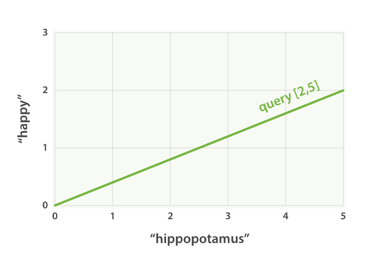
Imagine that we have a query for "happy hippopotamus". A common word like happy will have a low weight, while an uncommon term like hippopotamus will have a high weight. Let’s assume that happyhas a weight of 2 and hippopotamus has a weight of 5. We can plot this simple two-dimensional vector—[2,5]—as a line on a graph starting at point (0,0) and ending at point (2,5), as shown in Figure 27, “"happy hippopotamus" 를 나타내는 2차원 query vector”.
"happy hippopotamus" 를 검색한다고 가정해 보자. happy 같은 흔한 단어는 비중이 낮을 것이다. 반면에 hippopotamus 같이 흔하지 않은 단어는 비중이 높을 것이다. happy 는 2 라는 비중을 가지고, hippopotamus 는 5 라는 비중을 가진다고 가정해 보자. 이것으로, Figure 27, “"happy hippopotamus" 를 나타내는 2차원 query vector”과 같은, (0, 0)에서 시작하여 (2, 5)에서 끝나는 선 그래프인 이차원 vector [2, 5] 를 구성할 수 있다.
Now, imagine we have three documents:
이제, 3개의 document를 가정해 보자.
- I am happy in summer.
- After Christmas I’m a hippopotamus.
- The happy hippopotamus helped Harry.
We can create a similar vector for each document, consisting of the weight of each query term—happy and hippopotamus—that appears in the document, and plot these vectors on the same graph, as shown in Figure 28, “"happy hippopotamus"에 대한 query와 document vector”:
document에 나타나는 각 검색어(happy 와 hippopotamus)의 비중으로 구성되는, 각 document에 대한 유사한 vector를 생성할 수 있다. 그리고, 이들 vector로 Figure 28, “"happy hippopotamus"에 대한 query와 document vector”와 같은 그래프를 구성할 수 있다.
- Document 1:
(happy,____________)—[2,0] - Document 2:
( ___ ,hippopotamus)—[0,5] - Document 3:
(happy,hippopotamus)—[2,5]
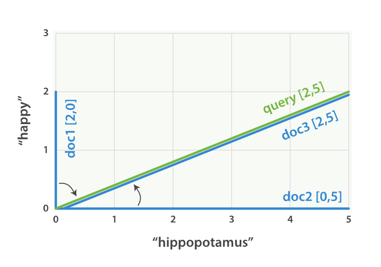
The nice thing about vectors is that they can be compared. By measuring the angle between the query vector and the document vector, it is possible to assign a relevance score to each document. The angle between document 1 and the query is large, so it is of low relevance. Document 2 is closer to the query, meaning that it is reasonably relevant, and document 3 is a perfect match.
vector의 좋은 점은 그들을 비교할 수 있다는 것이다. query vector와 document vector 사이의 각도를 측정함으로써, 각 document에 relevance score를 할당하는 것이 가능하다. document 1과 query사이의 각도는 크다. 그러므로 relevance가 낮다. document 2는 query에 더 가깝다. 즉, 상당히 관련 있다. 그리고, document 3은 완전히 일치한다.
In practice, only two-dimensional vectors (queries with two terms) can be plotted easily on a graph. Fortunately, linear algebra—the branch of mathematics that deals with vectors—provides tools to compare the angle between multidimensional vectors, which means that we can apply the same principles explained above to queries that consist of many terms.
실제로, 이차원 vector(2개의 단어로 된 query)만이 그래프를 쉽게 구성할 수 있다. 다행히도, 선형 대수학(linear algebra, vector를 다루는 수학의 일종)은 다차원 vector간의 각도를 비교할 수 있는 도구를 제공한다. 즉, 많은 단어로 구성된 query에 위에서 설명된 것과 동일한 원리를 적용할 수 있다.
You can read more about how to compare two vectors by using cosine similarity.
cosine similarity를 사용하여, 두 개의 vector를 비교하는 방법에 대하여 더 읽어 볼 수 있다.
Now that we have talked about the theoretical basis of scoring, we can move on to see how scoring is implemented in Lucene.
지금까지, score 계산의 이론적인 기초에 대해 이야기했고, 이제, Lucene에서 score 계산을 구현한 방법에 대해 이야기할 것이다.
'2.X > 2. Search in Depth' 카테고리의 다른 글
| 2-5-8. Ngrams for Compound Words (0) | 2017.09.24 |
|---|---|
| 2-6. Controlling Relevance (0) | 2017.09.24 |
| 2-6-02. Lucene’s Practical Scoring Function (0) | 2017.09.24 |
| 2-6-03. Query-Time Boosting (0) | 2017.09.24 |
| 2-6-04. Manipulating Relevance with Query Structure (0) | 2017.09.24 |