The other approximate metric offered by Elasticsearch is the percentiles metric. Percentiles show the point at which a certain percentage of observed values occur. For example, the 95th percentile is the value that is greater than 95% of the data.
Elasticsearch에 의해 제공되는 또 다른 approximate metric은, percentiles(백분위) metric이다.percentiles는 관찰된 값들 중에서 특정 비율이 나타나는 지점을 나타낸다. 예를 들어, 95번째 percentile는 데이터의 95%보다 더 큰 값이다.
Percentiles are often used to find outliers. In (statistically) normal distributions, the 0.13th and 99.87th percentiles represent three standard deviations from the mean. Any data that falls outside three standard deviations is often considered an anomaly because it is so different from the average value.
percentiles는 흔히 특이점을 발견하는데 사용한다. (통계적으로) 정규 분포에서, 0.13th과 99.87th의 percentiles는 평균의 세 가지 표준 편차를 나타낸다. 세 가지 표준 편차에 포함되지 않는 데이터는, 평균 값과 너무 다르기 때문에, 흔히 특이한 것으로 간주된다.
To be more concrete, imagine that you are running a large website and it is your job to guarantee fast response times to visitors. You must therefore monitor your website latency to determine whether you are meeting your goal.
좀 더 구체적으로, 아주 큰 website가 운영 중이고, 방문자에게 빠른 response 시간을 보장해 주는 것이 여러분의 업무라고 가정해 보자. 따라서, 목표의 충족 여부를 확인하기 위해, website의 대기 시간을 모니터링 해야 한다.
A common metric to use in this scenario is the average latency. But this is a poor choice (despite being common), because averages can easily hide outliers. A median metric also suffers the same problem. You could try a maximum, but this metric is easily skewed by just a single outlier.
이 시나리오에 사용하는 흔한 metric은 평균 대기 시간이다. 그러나, 평균(mean)에서는 특이 사항이 잘 나타나지 않기 때문에, 실제로는 좋지 않은 선택(일반적인데도 불구하고)이다. 중간 값(median) metric 또한 동일한 문제를 겪는다. 최대값(maximum)을 시도하겠지만, 이 metric은 하나의 특이 사항으로 쉽게 왜곡된다.
This graph in Figure 40, “시간별 request 평균 대기 시간” visualizes the problem. If you rely on simple metrics like mean or median, you might see a graph that looks like Figure 40, “시간별 request 평균 대기 시간”.
Figure 40, “시간별 request 평균 대기 시간”에 있는 그래프는 문제점을 보여준다. 평균(mean)이나 중간 값(median) 같은 단순한 metric을 사용한다면, Figure 40, “시간별 request 평균 대기 시간”과 같은 그래프를 볼 수 있을 것이다.
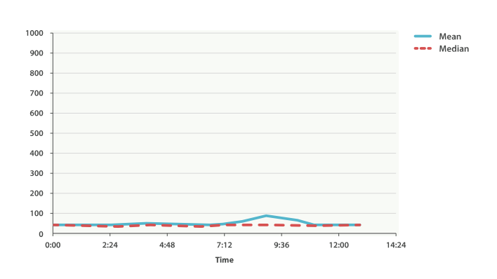
Everything looks fine. There is a slight bump, but nothing to be concerned about. But if we load up the 99th percentile (the value that accounts for the slowest 1% of latencies), we see an entirely different story, as shown in Figure 41, “시간에 따른 99th percentile 평균 대기 시간”.
모든 것이 정상이다. 약간 튀는 부분도 있지만, 염려할 것은 없다. 그러나, 99th percentile(대기 시간이 가장 느린 1%를 차지하는 값)을 알아보면, Figure 41, “시간에 따른 99th percentile 평균 대기 시간”에서 볼 수 있듯이, 완전히 다른 것을 알 수 있다.
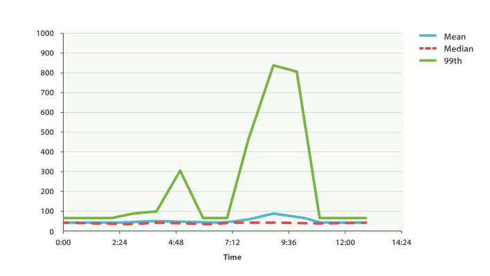
Whoa! At 9:30 a.m., the mean is only 75ms. As a system administrator, you wouldn’t look at this value twice. Everything normal! But the 99th percentile is telling you that 1% of your customers are seeing latency in excess of 850ms—a very different story. There is also a smaller spike at 4:48 a.m. that wasn’t even noticeable in the mean/median.
오전 9:30에, 평균은 겨우 75ms이다. 시스템 관리자로써, 이 값을 반복해서 보지 않을 것이다. 모든 것이 정상이다. 그러나, 99th percentile은 고객 중 1%의 대기 시간이 850ms를 초과한다고 알려준다. 전혀 다른 이야기이다. 오전 4:48에도 평균이나 중간 값에서는 전혀 눈에 띄지도 않는 작은 문제가 있었다.
This is just one use-case for a percentile. Percentiles can also be used to quickly eyeball the distribution of data, check for skew or bimodalities, and more.
이것은 percentiles 사용 사례 중의 하나이다. 데이터 분포를 빠르게 검토하거나, 왜곡, 이원화 등을 확인하는데 사용될 수 있다.
Percentile Metricedit
Let’s load a new dataset (the car data isn’t going to work well for percentiles). We are going to index a bunch of website latencies and run a few percentiles over it:
새로운 데이터 집합(자동차 데이터는 percentiles를 테스트하기에 적당하지 않다)을 만들어 보자. website의 대기 시간을 색인하고, 거기에 percentiles를 실행한다.
POST /website/logs/_bulk
{ "index": {}}
{ "latency" : 100, "zone" : "US", "timestamp" : "2014-10-28" }
{ "index": {}}
{ "latency" : 80, "zone" : "US", "timestamp" : "2014-10-29" }
{ "index": {}}
{ "latency" : 99, "zone" : "US", "timestamp" : "2014-10-29" }
{ "index": {}}
{ "latency" : 102, "zone" : "US", "timestamp" : "2014-10-28" }
{ "index": {}}
{ "latency" : 75, "zone" : "US", "timestamp" : "2014-10-28" }
{ "index": {}}
{ "latency" : 82, "zone" : "US", "timestamp" : "2014-10-29" }
{ "index": {}}
{ "latency" : 100, "zone" : "EU", "timestamp" : "2014-10-28" }
{ "index": {}}
{ "latency" : 280, "zone" : "EU", "timestamp" : "2014-10-29" }
{ "index": {}}
{ "latency" : 155, "zone" : "EU", "timestamp" : "2014-10-29" }
{ "index": {}}
{ "latency" : 623, "zone" : "EU", "timestamp" : "2014-10-28" }
{ "index": {}}
{ "latency" : 380, "zone" : "EU", "timestamp" : "2014-10-28" }
{ "index": {}}
{ "latency" : 319, "zone" : "EU", "timestamp" : "2014-10-29" }
This data contains three values: a latency, a data center zone, and a date timestamp. Let’s run percentiles over the whole dataset to get a feel for the distribution:
이 데이터는 3가지 값(대기 시간-latency, 데이터 센터의 지역-zone, timestamp)을 가지고 있다. 분포도를 얻기 위해, 전체 데이터 집합에 percentiles 를 실행해 보자.
GET /website/logs/_search { "size" : 0, "aggs" : { "load_times" : { "percentiles" : { "field" : "latency"} }, "avg_load_time" : { "avg" : { "field" : "latency"
} } } }
|
|
| 비교하기 위해, 동일한 field에 |
By default, the percentiles metric will return an array of predefined percentiles: [1, 5, 25, 50, 75, 95, 99]. These represent common percentiles that people are interested in—the extreme percentiles at either end of the spectrum, and a few in the middle. In the response, we see that the fastest latency is around 75ms, while the slowest is almost 600ms. In contrast, the average is sitting near 200ms, which is much less informative:
기본적으로, percentiles metric은 미리 정의된 percentiles의 배열([1, 5, 25, 50, 75, 95, 99])을 반환한다. 이것은 사람들이 관심을 가지는, 일반적인 percentiles(스펙트럼의 끝, 중간의 몇 개중에 극단적인 percentiles)를 나타낸다. response에서 가장 빠른 대기 시간은 약 75ms이다. 반면에 가장 느린 response 시간은 거의 600ms이다. 반대로, 평균은 거의 200ms이다. 거의 도움이 되지 않는다.
...
"aggregations": {
  "load_times": {
     "values": {
        "1.0": 75.55,
        "5.0": 77.75,
        "25.0": 94.75,
        "50.0": 101,
        "75.0": 289.75,
        "95.0": 489.34999999999985,
        "99.0": 596.2700000000002
     }
  },
  "avg_load_time": {
     "value": 199.58333333333334
  }
}
So there is clearly a wide distribution in latencies. Let’s see whether it is correlated to the geographic zone of the data center:
따라서, 대기 시간에는 분명히 넓은 분포가 있다. 데이터센터의 지리적 위치(zone)와 상관관계가 있는지 알아보자.
GET /website/logs/_search { "size" : 0, "aggs" : { "zones" : { "terms" : { "field" : "zone"} }, "load_avg" : { "avg" : { "field" : "latency" } } } } } }
| 먼저, zone에 따라 latency를 bucket으로 분리한다. |
| 그 다음에 zone별로 percentiles를 계산한다. |
|
|
From the response, we can see the EU zone is much slower than the US zone. On the US side, the 50th percentile is very close to the 99th percentile—and both are close to the average.
response에서, EU 지역이 US 지역보다 훨씬 더 느린 것을 알 수 있다. US 지역에서는 50th percentile이 99th percentile에 거의 근접해 있다. 그리고, 모두 평균에 가깝다.
In contrast, the EU zone has a large difference between the 50th and 99th percentile. It is now obvious that the EU zone is dragging down the latency statistics, and we know that 50% of the EU zone is seeing 300ms+ latencies.
반면에, EU 지역은 50th과 99th percentile 사이에 큰 차이가 있다. EU 지역이 대기 시간(latency) 통계를 끌어 내리고 있는 것은 분명하다. EU 지역 50%의 대기 시간이 300ms 이상인 것을 알 수 있다.
...
"aggregations": {
  "zones": {
     "buckets": [
        {
           "key": "eu",
           "doc_count": 6,
           "load_times": {
              "values": {
                 "50.0": 299.5,
                 "95.0": 562.25,
                 "99.0": 610.85
              }
           },
           "load_avg": {
              "value": 309.5
           }
        },
        {
           "key": "us",
           "doc_count": 6,
           "load_times": {
              "values": {
                 "50.0": 90.5,
                 "95.0": 101.5,
                 "99.0": 101.9
              }
           },
           "load_avg": {
              "value": 89.66666666666667
           }
        }
     ]
  }
}
...
Percentile Ranksedit
There is another, closely related metric called percentile_ranks. The percentiles metric tells you the lowest value below which a given percentage of documents fall. For instance, if the 50th percentile is 119ms, then 50% of documents have values of no more than 119ms. The percentile_ranks tells you which percentile a specific value belongs to. The percentile_ranks of 119ms is the 50th percentile. It is basically a two-way relationship. For example:
percentile_ranks 라 불리는, 밀접하게 연관된 또 하나의 metric이 있다. percentiles metric은 주어진 document의 비율 아래에 가장 낮은 값을 알려준다. 예를 들어, 50th percentile이 119ms 이면, document의 50%는 119ms 보다 더 큰 값을 가지지 않는다. percentile_ranks 는 특정 값에 해당하는 percentile을 알려준다. 119ms 의 percentile_ranks 는 50th percentile이다. 기본적으로 양방향 관계이다. 예를 들면,
The 50th percentile is 119ms.
50th percentile은 119ms 이다.
The 119ms percentile rank is the 50th percentile.
119ms 의 percentile rank는 50th percentile이다.
So imagine that our website must maintain an SLA of 210ms response times or less. And, just for fun, your boss has threatened to fire you if response times creep over 800ms. Understandably, you would like to know what percentage of requests are actually meeting that SLA (and hopefully at least under 800ms!).
website가 response 시간 210ms 이하의 SLA(서비스 수준 협약서, Service Level Agreement)를 유지해야 하고, 재미를 위해서, 관리자가 response 시간이 800ms 이상이면 해고한다는 협박을 하고 있다고 가정해 보자. 여러분은 당연히 SLA를 충족시키는 (최소한 800ms 이하일 거라는 희망을 가지고) request의 비율을 알고 싶을 것이다.
For this, you can apply the percentile_ranks metric instead of percentiles:
이를 위해, percentiles 대신에 percentile_ranks metric을 적용할 수 있다.
GET /website/logs/_search { "size" : 0, "aggs" : { "zones" : { "terms" : { "field" : "zone" }, "aggs" : { "load_times" : { "percentile_ranks" : { "field" : "latency", "values" : [210, 800]
|
|
After running this aggregation, we get two values back:
이 aggregation을 실행한 후에, 두 가지 값을 얻을 수 있다.
"aggregations": {
  "zones": {
     "buckets": [
        {
           "key": "eu",
           "doc_count": 6,
           "load_times": {
              "values": {
                 "210.0": 31.944444444444443,
                 "800.0": 100
              }
           }
        },
        {
           "key": "us",
           "doc_count": 6,
           "load_times": {
              "values": {
                 "210.0": 100,
                 "800.0": 100
              }
           }
        }
     ]
  }
}
This tells us three important things:
여기에서 3가지 중요한 점을 알 수 있다.
In the EU zone, the percentile rank for 210ms is 31.94%.
EU 지역에서, 210ms 에 대한 percentile rank는 31.94% 이다.
In the US zone, the percentile rank for 210ms is 100%.
US 지역에서, 210ms 에 대한 percentile rank는 100% 이다.
In both EU and US, the percentile rank for 800ms is 100%.
EU, US 양쪽 지역에서, 800ms 에 대한 percentile rank는 100% 이다.
In plain english, this means that the EU zone is meeting the SLA only 32% of the time, while the US zone is always meeting the SLA. But luckily for you, both zones are under 800ms, so you won’t be fired (yet!).
쉽게 말하면, EU 지역은 SLA의 32% 만을 만족시키는데, US 지역은 항상 SLA를 만족시킨다. 그러나, 다행스럽게도, 양쪽 지역 모두 800ms 아래이다. 그래서 해고되지 않을 것이다.(아직은!)
The percentile_ranks metric provides the same information as percentiles, but presented in a different format that may be more convenient if you are interested in specific value(s).
percentile_ranks metric은 percentiles 와 동일한 정보를 제공한다. 그러나 특정 값(들)에 관심이 있다면, 더 편리할 수 있는 다른 형식으로 나타난다.
Understanding the Trade-offsedit
Like cardinality, calculating percentiles requires an approximate algorithm. The naiveimplementation would maintain a sorted list of all values—but this clearly is not possible when you have billions of values distributed across dozens of nodes.
cardinality와 마찬가지로, percentiles의 계산은 approximate 알고리즘을 필요로 한다. 단순하게 구현하면, 모든 값의 정렬된 목록을 유지하는 것이다. 하지만, 수십 개의 node에 분산된 수십억 개의 값을 가지고 있을 경우, 이것은 분명히 불가능하다.
Instead, percentiles uses an algorithm called TDigest (introduced by Ted Dunning in Computing Extremely Accurate Quantiles Using T-Digests). As with HyperLogLog, it isn’t necessary to understand the full technical details, but it is good to know the properties of the algorithm:
대신, percentiles 는 TDigest(Computing Extremely Accurate Quantiles Using T-Digests에서 Ted Dunning에 의해 소개된)라 불리는 알고리즘을 사용한다. HyperLogLog와 마찬가지로, 기술적인 세부사항 전체를 이해할 필요는 없다. 그러나, 알고리즘의 특성을 알고 있는 것이 좋다.
Percentile accuracy is proportional to how extreme the percentile is. This means that percentiles such as the 1st or 99th are more accurate than the 50th. This is just a property of how the data structure works, but it happens to be a nice property, because most people care about extreme percentiles.
percentile의 정밀도는 percentile가 얼마나 극단적(extreme) 인가에 비례한다. 즉, 1st 나 99th 같은 percentiles는 50th 보다 더 정확하다. 이것은 단지 데이터 구조가 동작하는 방법의 특성이지만, 대부분의 사람들은 극단적인 percentiles에 대해 주의하기 때문에, 좋은 특성이 된다.
For small sets of values, percentiles are highly accurate. If the dataset is small enough, the percentiles may be 100% exact.
값이 작은 집합일 경우, percentiles는 매우 정확하다. 데이터 집합이 충분히 작으면, percentiles는 100% 정확할 것이다.
As the quantity of values in a bucket grows, the algorithm begins to approximate the percentiles. It is effectively trading accuracy for memory savings. The exact level of inaccuracy is difficult to generalize, since it depends on your data distribution and volume of data being aggregated.
bucket에 있는 값의 양이 증가함에 따라, 알고리즘은 percentiles에 근접하기 시작한다. 효과적으로 정확성을 메모리 절약과 교환한다. 부정확성의 정확한 수준은, aggregation될 데이터의 분포나 데이터의 양에 따라 달라지기 때문에, 일반화하기 어렵다.
Similar to cardinality, you can control the memory-to-accuracy ratio by changing a parameter: compression.
cardinality 와 마찬가지로, compression 매개변수를 변경하여, 메모리와 정확성의 비율을 제어할 수 있다.
The TDigest algorithm uses nodes to approximate percentiles: the more nodes available, the higher the accuracy (and the larger the memory footprint) proportional to the volume of data. The compression parameter limits the maximum number of nodes to 20 * compression.
TDigest 알고리즘은 approximate percentiles에, node의 수를 사용한다. 이용할 수 있는 node가 많을수록, 데이터의 양에 비례하여, 정확성(과 큰 메모리 공간)이 더 높다. compression 매개변수는, 20 * compression 로, 최대 node 수를 제한한다.
Therefore, by increasing the compression value, you can increase the accuracy of your percentiles at the cost of more memory. Larger compression values also make the algorithm slower since the underlying tree data structure grows in size, resulting in more expensive operations. The default compression value is 100.
따라서, compression 값을 증가시킴으로써, 더 많은 메모리 비용으로, percentiles의 정확성을 증가시킬 수 있다. 더 큰 compression 값은 기본 tree 데이터 구조의 크기를 증가시켜, 더 비싼 연산으로 나타나기 때문에, 알고리즘을 느리게 만든다. compression의 기본 값은 100 이다.
A node uses roughly 32 bytes of memory, so in a worst-case scenario (for example, a large amount of data that arrives sorted and in order), the default settings will produce a TDigest roughly 64KB in size. In practice, data tends to be more random, and the TDigest will use less memory.
어떤 node가 대략 32 byte의 메모리를 사용한다면, 최악의 시나리오(정리정돈되어 도착한 많은 양의 데이터)에서, 기본 설정은 64KB 정도로 TDigest를 생성한다. 실제에서 데이터는 더 무작위이고, TDigest는 더 적은 메모리를 사용할 것이다.
'2.X > 4. Aggregations' 카테고리의 다른 글
| 4-08. Approximate Aggregations (0) | 2017.09.23 |
|---|---|
| 4-08-1. Finding Distinct Counts (0) | 2017.09.23 |
| 4-09. Significant Terms (0) | 2017.09.23 |
| 4-09-1. significant_terms Demo (0) | 2017.09.23 |
| 4-10. Doc Values and Fielddata (0) | 2017.09.23 |