In the previous blog post, “Time Series Data and MongoDB: Part 1 – An Introduction,” we introduced the concept of time-series data followed by some discovery questions you can use to help gather requirements for your time-series application. Answers to these questions help guide the schema and MongoDB database configuration needed to support a high-volume production application deployment. In this blog post we will focus on how two different schema designs can impact memory and disk utilization under read, write, update, and delete operations.
이전 게시물인 “Time Series Data and MongoDB: Part 1 – An Introduction”에서, 시계열 data의 개념을 소개하고, 시계열 application의 요규사항을 수집하는데 도움이 되는 몇 가지 질물을 소개했다. 이들 질문에 대한 답변은 대용량 application의 배포를 지원하는데 필요한 schema와 MongoDB database 구성에 도움이 된다. 이 게시물에서는, read, write, update, delete 연산에서 2가지 다른 schema design이 memory와 disk 사용률에 얼마나 영향을 미치는지에 대해 중점적으로 다룰것이다.
In the end of the analysis you may find that the best schema design for your application may be leveraging a combination of schema designs. By following the recommendations we lay out below, you will have a good starting point to develop the optimal schema design for your app, and appropriately size your environment.
분석이 끝나면 application에 가장 적합한 scheman design은 schema design의 조합을 활용하는 것이라는 것을 발견할 것이다. 아래에 제시한 권장사항을 따르면, 여러분의 app에 최적인 schema design을 개발하고, 여러분의 환경에 적절히 조절할 수 있는 좋은 출발점이 될 것이다.
Designing a time-series schema
Let’s start by saying that there is no one canonical schema design that fits all application scenarios. There will always be trade-offs to consider regardless of the schema you develop. Ideally you want the best balance of memory and disk utilization to yield the best read and write performance that satisfy your application requirements, and that enables you to support both data ingest and analysis of time-series data streams.
먼저, 모든 application 시나리오에 적합한 표준 schema design은 없다는 점부터 시작하자. 개발하려는 schema에 관계없이 항상 고려해야 할 trade-offs가 있다. 이상적으로는 application 요구사항을 만족시키고, data 수집과 시계열 data stream의 분석을 동시에 지원할 수 있는, 최상의 read, write 성능을 충족시키기 위해, 최적의 memory 및 disk 사용량의 균형을 원한다.
In this blog post we will look at various schema design configurations. First, storing one document per data sample, and then bucketing the data using one document per time-series time range and one document per fixed size. Storing more than one data sample per document is known as bucketing. This will be implemented at the application level and requires nothing to be configured specifically in MongoDB. With MongoDB’s flexible data model you can optimally bucket your data to yield the best performance and granularity for your application’s requirements.
이 게시물에서, 다양한 schema design 구성을 살펴볼 것이다. 먼저, data 샘플 당 하나의 document를 저장한 다음, 시계열 시간 범위당 하나의 document와 고정된 크기당 하나의 document를 사용하여, data를 bucketing한다. document당 하나 이상의 data 샘플을 저장하는 것을 bucketing이라 한다. 이것은 application 수준에서 구현되며, MongoDB에서 특별히 구성해야 할 필요는 없다. MongoDB의 유연한 data model을 사용하면 data를 최적의 상태로 bucket에 배치하여, application의 요구사항에 맞는 최상의 성능과 세분성을 얻을 수 있다.
This flexibility also allows your data model to adapt to new requirements over time – such as capturing data from new hardware sensors that were not part of the original application design. These new sensors provide different metadata and properties than the sensors you used in the original design. With all this flexibility you may think that MongoDB databases are the wild west, where anything goes and you can quickly end up with a database full of disorganized data. MongoDB provides as much control as you need via schema validation that allows you full control to enforce things like the presence of mandatory fields and range of acceptable values, to name a few.
또한, 이러한 유연성으로 인해, data model을 시간에 따른 새로운 요구 사항(원래의 application design의 일부가 아닌 새로운 HW sensor에서 data를 얻는 것 같은)에 맞게 조정할 수 있다. 이러한 새로운 sensor는 원래의 design에서 사용된 sensor와 다른 metadata와 속성을 제공한다. 이러한 유연성 때문에 MongoDB database는 어떤 일이든 가능하며, 체계적이지 않은 data로 가드찬 database를 쉽게 구축할 수 있다고 생각할 수 있다. MongoDB는 schema validation을 통해 필요한 만큼 제어할 수 있으며, 이를 통해 필수 field가 있는지, 허용 값의 범위 같은 것들을 강제할 수 있도록 완전한 제어가 가능하다.
To help illustrate how schema design and bucketing affects performance, consider the scenario where we want to store and analyze historical stock price data. Our sample stock price generator application creates sample data every second for a given number of stocks that it tracks. One second is the smallest time interval of data collected for each stock ticker in this example. If you would like to generate sample data in your own environment, the StockGen tool is available on GitHub. It is important to note that although the sample data in this document uses stock ticks as an example, you can apply these same design concepts to any time-series scenario like temperature and humidity readings from IoT sensors.
schema design과 bucketing이 성능에 미치는 영향을 설명하기 위해, 과거의 주식 가격 data를 저장하고 분석하는 시나리오를 생각해 보자. 샘플 주식 가격 생성 application은 그것이 추적하는 정해진 수의 주식에 대해 매초마다 샘플 data를 생성한다. 1초는 이 예제에서 각 주식 시세에 대해 수집된 data의 최소 시간 간격이다. 여러분이 셈플 data를 생성하려면, GitHub에서 StockGen tool을 사용할 수 있다. 이 document의 샘플 data는 주식 ticks를 예제로 사용하지만, IoT sensor의 온도와 습도 판독값 같은 어떤 시계열 시나리오에도 이런 동일한 design 개념을 적용할 수 있다는 점을 기억하자.
The StockGen tool used to generate sample data will generate the same data and store it in two different collections: StockDocPerSecond and StockDocPerMinute that each contain the following schemas:
sample data를 생성하는데 사용되는 StocGen tool은 2개의 다른 collection에 동일한 data를 생성해 저장한다. StockDocPerSecond와 StockDocPerMinute 각각은 다음과 같은 schema를 가진다.
Scenario 1: One document per data point
{
  "_id" : ObjectId("5b4690e047f49a04be523cbd"),
"p" : 56.56,
  "symbol" : "MDB",
  "d" : ISODate("2018-06-30T00:00:01Z")
},
{
  "_id" : ObjectId("5b4690e047f49a04be523cbe"),
"p" : 56.58,
  "symbol" : "MDB",
  "d" : ISODate("2018-06-30T00:00:02Z")
}
,...
Scenario 2: Time-based bucketing of one document per minute
{
"_id" : ObjectId("5b5279d1e303d394db6ea0f8"),
"p" : {
"0" : 56.56,
"1" : 56.56,
"2" : 56.58,
…
"59" : 57.02
},
"symbol" : "MDB",
"d" : ISODate("2018-06-30T00:00:00Z")
},
{
"_id" : ObjectId("5b5279d1e303d394db6ea134"),
"p" : {
 "0" : 69.47,
 "1" : 69.47,
 "2" : 68.46,
...
 "59" : 69.45
},
"symbol" : "TSLA",
"d" : ISODate("2018-06-30T00:01:00Z")
},...
Note that the field “p” contains a subdocument with the values for each second of the minute.
“p” field는 해당 분의 각 초에 대한 값을 가지는 하위 document를 포함한다.
Schema design comparisons
Let’s compare and contrast the database metrics of storage size and memory impact based off of 4 weeks of data generated by the StockGen tool. Measuring these metrics is useful when assessing database performance.
StocGen tool로 생성된 4주 분량의 data를 기반으로 저장소 크기와 memory 영향에 대한 database metric을 비교하고 대조해 보자. 이들 metric을 측정하는 것은 database의 성능을 평가할 때 유용하다.
Effects on Data Storage
In our application the smallest level of time granularity is a second. Storing one document per second as described in Scenario 1 is the most comfortable model concept for those coming from a relational database background. That is because we are using one document per data point, which is similar to a row per data point in a tabular schema. This design will produce the largest number of documents and collection size per unit of time as seen in Figures 3 and 4.
이 application에서 가장 작은 수준의 시간 세분화는 2번째이다. 시나리오 1에 설명한 대로, 초당 하나의 document를 저장하는 것이 RDB 관점에서 보면 가장 익숙한 모델이다. 표(table) 형식 schema에서 data별로 하나의 row와 유사하게, data별로 하나의 document를 사용하기 때문이다.

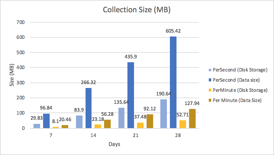
Figure 4 shows two sizes per collection. The first value in the series is the size of the collection that is stored on disk, while the second value is the size of the data in the database. These numbers are different because MongoDB’s WiredTiger storage engine supports compression of data at rest. Logically the PerSecond collection is 605MB, but on disk it is consuming around 190 MB of storage space.
그림4는 collection별로 2개의 크기를 보여준다. 첫번째 값은 disk에 저장된 collection의 크기이고, 두번째 값은 database의 data 크기이다. MongoDb의 WiredTiger storage engine은 미사용 data의 compression을 지원하기 때문에, 이들 숫자는 다르다. 이론적으로 PerSecond collect은 650MB 이지만, disk에서는 약 190MB 의 저장소 공간을 소비한다.
Effects on memory utilization
A large number of documents will not only increase data storage consumption but increase index size as well. An index was created on each collection and covered the symbol and date fields. Unlike some key-value databases that position themselves as time-series databases, MongoDB provides secondary indexes giving you flexible access to your data and allowing you to optimize query performance of your application.
많은 수의 document는 data 저장소뿐만 아니라 index 크기도 증가시킨다. index는 각 collection 별로 생성되고, 기호 및 date field를 포함한다. 스스로를 시계열 database라 하는 일부 key-value database와 달리, MongoDB는 secondary indexes 를 제공하여, data의 유연한 access와 application에서의 query 성능 최적화가 가능하다.
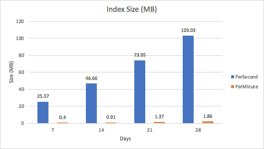
The size of the index defined in each of the two collections IS seen in Figure 5. Optimal performance of MongoDB happens when indexes and most recently used documents fit into the memory allocated by the WiredTiger cache (we call this the “working set”). In our example we generated data for just 5 stocks over the course of 4 weeks. Given this small test case our data already generated an index that is 103MB in size for the PerSecond scenario. Keep in mind that there are some optimizations such as index prefix compression that help reduce the memory footprint of an index. However, even with these kind of optimizations proper schema design is important to prevent runaway index sizes. Given the trajectory of growth, any changes to the application requirements, like tracking more than just 5 stocks or more than 4 weeks of prices in our sample scenario, will put much more pressure on memory and eventually require indexes to page out to disk. When this happens your performance will be degraded. To mitigate this situation, consider scaling horizontally.
2 collection 각각에 정의된 index의 크기는 그림5에서 볼 수 있다. MongoDB의 최적 성능은 index와 가장 최근 사용된 document가 WiredTiger cache(우리는 이를 "working set"이라 한다)에 할당된 memory에 적합할 경우에 발생한다. 이 예에서 4주동안 5개의 주식에 대한 data를 생성했다. 이 작은 테스트에서, 이 data는 PerSecond 시나리오에 대해 크기가 103MB인 index를 생성했다. index의 memory 공간을 줄이는데 도움이 되는 index prefix compression 같은 최적화가 있음을 기억하자. 그러나, 이런 종류의 최적화에도 불구하고, index 크기의 급증을 방지하기 위하여 적절한 schema design이 중요하다. 증가 추이를 고려하여, 샘플 시나리오에서 5개 이상의 주식 또는 4주 이상의 가격을 추적하는 것 같은, application 요구사항의 변경은 memory에 더 많은 부담을 줄 것이고, 결국 index가 disk에 paging될 것이다. 이렇게 되면 성능히 저하될 것이다. 이 상황을 피하려면, 수평확장을 고려하자.
Scale horizontally
As your data grows in size you may end up scaling horizontally when you reach the limits of the physical limits of the server hosting the primary mongod in your MongoDB replica set.
data 크기가 증가하면, MongoDB replica set에서 primary momgod을 가지는 server의 물리적 한계에 도달하면, 결국 수평확장 해야 한다.
By horizontally scaling via MongoDB Sharding, performance can be improved since the indexes and data will be spread over multiple MongoDB nodes. Queries are no longer directed at a specific primary node. Rather they are processed by an intermediate service called a query router (mongos), which sends the query to the specific nodes that contain the data that satisfy the query. Note that this is completely transparent to the application – MongoDB handles all of the routing for you
MongoDB Sharding을 통해 수평확장을 하면, index와 data가 MongoDB node에 분산되므로, 성능은 향상된다. query는 더 이상 특정 primary node로 전달되지 않는다. 오히려 그것들은 query router(mongos)라는 중간 서비스에 의해 처리되는데, 이것은 query를 충족시키는 data를 가진 특정 node로 query를 전송한다.이것은 application과 완전히 분리되어 있다는 점을 기억하자. MongoDB가 모든 routing을 처리한다.
Scenario 3: Size-based bucketing
The key takeaway when comparing the previous scenarios is that bucketing data has significant advantages. Time-based bucketing as described in scenario 2 buckets an entire minute's worth of data into a single document. In time-based applications such as IoT, sensor data may be generated at irregular intervals and some sensors may provide more data than others. In these scenarios, time-based bucketing may not be the optimal approach to schema design. An alternative strategy is size-based bucketing. With size-based bucketing we design our schema around one document per a certain number of emitted sensor events, or for the entire day, whichever comes first.
이전 시나리오와 비교할 때 중요한 점은 bucketing data는 상당한 이점을 가진다는 것이다. 시나리오 2에서 설명한 시계열 bucketing은 전체 분(minute)의 data를 단일 document로 bucket화 한다. IoT 같은 시계열 application에서, sensor data가 불규칙한 시간으로 생성될 수 있고, 일부 sensor는 다른 것보다 더 많은 data를 제공할 수 있다. 이 시나리오에서, 시계열 bucketing은 schema design에 대한 최적의 방법이 아닐 수 있다. 대안은 크기 기반 bucketing이다. 크기 기반 bucketing을 사용하여, 출력된 sensor event의 특정 횟수 별로 또는 또는 전체 날짜에 대해 먼저 발생하는 것을 하나의 document로 schema를 design한다.
To see size-based bucketing in action, consider the scenario where you are storing sensor data and limiting the bucket size to 200 events per document, or a single day (whichever comes first). Note: The 200 limit is an arbitrary number and can be changed as needed, without application changes or schema migrations.
크기 기반 bucketing을 보려면, sensor data를 저장하고, bucket 크기를 document당 200 event 또는 하루(먼저 발생하는)로 제한하는 시나리오를 고려하자. 200이라는 제한은 임의의 숫자이며, application의 변경이나 schema migration 없이, 필요에 따라 변경될 수 있다.
{
  _id: ObjectId(),
 deviceid: 1234,
 sensorid: 3,
 nsamples: 5,
  day: ISODate("2018-08-29"),
 first:1535530412,
 last: 1535530432,
 samples : [
   { val: 50, time: 1535530412},
   { val: 55, time : 1535530415},
   { val: 56, time: 1535530420},
   { val: 55, time : 1535530430},
   { val: 56, time: 1535530432}
   ]
}
An example size-based bucket is shown in figure 6. In this design, trying to limit inserts per document to an arbitrary number or a specific time period may seem difficult; however, it is easy to do using an upsert, as shown in the following code example:
크기 기반 bucket의 예는 그림 6에서 볼 수 있다. 이 design에서, document 별로 임의의 숫자나 특정 시간 간격으로 insert를 제한하는 것이 어려워보일 수 있다. 그러나, 다음 code 예제와 같이 upsert를 사용하면 쉽다.
sample = {val: 59, time: 1535530450}
day = ISODate("2018-08-29")
db.iot.updateOne({deviceid: 1234, sensorid: 3, nsamples: {$lt: 200}, day: day},
                 {$push: {samples: sample},
                  $min: {first: sample.time},
                  $max: {last: sample.time},
                  $inc: {nsamples: 1}, {upsert: true} )
As new sensor data comes in it is simply appended to the document until the number of samples hit 200, then a new document is created because of our upsert:true clause.
새로운 sensor data가 들어오면, sample 수가 200개가 될 때까지 추가된다. 그 다음에 upsert:true 절 때문에 새로운 document가 추가된다.
The optimal index in this scenario would be on {deviceid:1,sensorid:1,day:1,nsamples:1}. When we are updating data, the day is an exact match, and this is super efficient. When querying we can specify a date, or a date range on a single field which is also efficient as well as filtering by first and last using UNIX timestamps. Note that we are using integer values for times. These are really times stored as a UNIX timestamp and only take 32 bits of storage versus an ISODate which takes 64 bits. While not a significant query performance difference over ISODate, storing as UNIX timestamp may be significant if you plan on ending up with terabytes of ingested data and you do not need to store a granularity less than a second.
이 시나리오에서 최적의 index는 {deviceid:1,sensorid:1,day:1,nsamples:1} 이다. data를 update할 경우, day가 정확한 일치이며, 이것은 매우 효율적이다. query시에, UNIX timestamp를 사용하여 처음과 마지막을 filtering하는 것과 마찬가지로 date나 date 범위를 단일 filed에 지정하는데, 이 또한 효율적이다.시간 값에 대해 integer를 사용한다는 점을 기억하자. 이것은 실제 시간을 UNIX timestamp로 저장하는 것이고, ISODate가 64bit를 사용하는 것에 비해, 32bit 저장소만 사용한다.ISODate에 비해 현저한 query 성능 차이는 아니지만, 수 TB의 data를 수집하고, 1초 미만의 자세한 data를 저장할 필요가 없다면, UNIX timestamp로 저장하는 것은 의미가 있다.
Bucketing data in a fixed size will yield very similar database storage and index improvements as seen when bucketing per time in scenario 2. It is one of the most efficient ways to store sparse IoT data in MongoDB.
고정된 크기의 data를 bucketing하면, 시나리오 2에서 시간별로 bucketing하는 경우와 매우 유사한 database 저장소와 index 개선을 보인다. MongoDB에서 희박한 IoT data를 저장하는 가장 효율적인 방법 중 하나이다.
What to do with old data
Should we store all data in perpetuity? Is data older than a certain time useful to your organization? How accessible should older data be? Can it be simply restored from a backup when you need it, or does it need to be online and accessible to users in real time as an active archive for historical analysis? As we covered in part 1 of this blog series, these are some of the questions that should be asked prior to going live.
모든 data를 영구 저장해야 하는가? 특정 시간보다 오래된 data가 귀사에 유용한가? 이전 data에 어떻게 access 가능해야 하는가? 필요할 경우 backup에서 간단하게 복원되어야 하는가? 아니면, online이어야 하고, 사용자가 실시간 이력 분석을 위해 활성화된 archive에 access할 수 있어야 하는가? 이 게시물의 part 1에서 다루었듯이, 이런 것들이 실제 상황으로 가기 전에 질문해야 할 몇 가지 질문이다.
There are multiple approaches to handling old data and depending on your specific requirements some may be more applicable than others. Choose the one that best fits your requirements.
이전 data를 처리하는데에는 몇 가지 방법이 있으며, 구체적인 요구 사항에 따라, 몇 가지는 다른 것보다 더 적합할 수도 있다. 요구 사항에 가장 적합한 것을 고르자.
Pre-aggregation
Does your application really need a single data point for every event generated years ago? In most cases the resource cost of keeping this granularity of data around outweighs the benefit of being able to query down to this level at any time. In most cases data can be pre-aggregated and stored for fast querying. In our stock example, we may want to only store the closing price for each day as a value. In most architectures, pre-aggregated values are stored in a separate collection since typically queries for historical data are different than real-time queries. Usually with historical data, queries are looking for trends over time versus individual real-time events. By storing this data in different collections you can increase performance by creating more efficient indexes as opposed to creating more indexes on top of real-time data.
몇 년전에 생성된 모든 event에 대한 단일 data point가 application에 정말 필요한가? 대부분의 경우, 이러한 세분화된 data를 유지하는데 드는 resource 비용은 항상 이런 수준으로 query할 수 있을 때의 이점보다 크다. 대부분의 경우, 빠른 query를 위해 data를 사전 집계하여 저장할 수 있다. 주식 예제에서, 매일 마감 가격만을 값으로 저장하려 할 수도 있다. 일반적으로 과거 data에 대한 query는 실시간 query와 다르므로, 사전 집계 값들은 별도의 collection에 저장된다. 일반적으로, 과거 data의 경우, query는 실시간 event에 비해 시간별 추세를 찾는다. 다른 collection에 이 data를 저장하면, 실시간 data에 더 많은 index를 생성하는 것이 아니라 보다 효율적인 index를 생성함으로써, 성능을 향상시킬 수 있다.
Offline archival strategies
When data is archived, what is the SLA associated with retrieval of the data? Is restoring a backup of the data acceptable or does the data need to be online and ready to be queried at any given time? Answers to these questions will help drive your archive design. If you do not need real-time access to archival data you may want to consider backing up the data and removing it from the live database. Production databases can be backed up using MongoDB Ops Manager or if using the MongoDB Atlas service you can use a fully managed backup solution.
data를 archive하면, data의 검색과 관련된 SLA는? backup data를 복원이 허용되어야 하는가? 또는 data는 online이어야 하고 특정 시점에 query될 준비가 되어 있어야 하는가? 이 질문에 대한 답변은 archive design을 추친하는데 도움이 될 것이다. archive data에 대한 실시간 access가 필요하지 않다면, data를 backup하고, live database에서 제거하는 것을 고려해 보자. production database는 MongoDB Ops Manager를 사용하여 backup할 수 있으며, MongoDB Atlas service를 사용한다면, 완벽하게 관리되는 backup solution을 사용할 수 있다.
Removing documents using remove statement
Once data is copied to an archival repository via a database backup or an ETL process, data can be removed from a MongoDB collection via the remove statement as follows:
data가 database backup이나 ETL process를 통해 archive repository에 복사되면, 다음과 같이 remove 명령어를 통해 MongoDB collection에서 data를 제거할 수 있다.
db.StockDocPerSecond.remove ( { "d" : { $lt: ISODate( "2018-03-01" ) } } )In this example all documents that have a date before March 1st, 2018 defined on the “d” field will be removed from the StockDocPerSecond collection.
이 예제에서, "d" field에 2018년 3월 1일 이전의 날짜를 가지고 있는 모든 document는 StockDocPerSecond collection에서 제거된다.
You may need to set up an automation script to run every so often to clean out these records. Alternatively, you can avoid creating automation scripts in this scenario by defining a time to live (TTL) index.
이들 record를 정리하기 위해 주기적으로 자주 실행되는 자동화 script를 설정해야 할 수도 있다. 또는, TTL index를 정의하여, 이 시나리오에서 자동화 script를 생성하지 않을 수 있다.
Removing documents using a TTL Index
A TTL index is similar to a regular index except you define a time interval to automatically remove documents from a collection. In the case of our example, we could create a TTL index that automatically deletes data that is older than 1 week.
TTL index 는 collection에서 document를 자동으로 제거하는 시간을 정의한다는 점을 제외하면, 일반 index와 유사하다. 예제에서, TTL index를 생성하여, 1주일 이상 경과된 data를 자동으로 삭제한다.
db.StockDocPerSecond.createIndex( { "d": 1 }, { expireAfterSeconds: 604800 } )Although TTL indexes are convenient, keep in mind that the check happens every minute or so and the interval cannot be configured. If you need more control so that deletions won’t happen during specific times of the day you may want to schedule a batch job that performs the deletion in lieu of using a TTL index.
TTL index는 편리하지만, 매 분(minute)마다 점검해야 하고, 간격을 설정할 수 없다는 점을 기억하자. 하루 중 특정 시간대에 삭제가 발생하지 않도록 더 많은 제어가 필요하다면, TTL index를 사용하는 대신 삭제를 수행하는 batch job을 예약하자.
Removing documents by dropping the collection
It is important to note that using the remove command or TTL indexes will cause high disk I/O. On a database that may be under high load already this may not be desirable. The most efficient and fastest way to remove records from the live database is to drop the collection. If you can design your application such that each collection represents a block of time, when you need to archive or remove data all you need to do is drop the collection. This may require some smarts within your application code to know which collections should be queried, but the benefit may outweigh this change. When you issue a remove, MongoDB also has to remove data from all affected indexes as well and this could take a while depending on the size of data and indexes.
remove command나 TTL index를 사용하면 많은 disk I/O가 발생한다는 점에 유의하자. 이미 많은 부하가 있을 수도 있는 database에 이것은 바람직하지 않다. live database에서 record를 제거하는 가장 효율적이고 빠른 방법은 collection을 삭제하는 것이다. 각 collection이 시간을 나타내도록 application을 design할 수 있다면, data를 archive하거나 제거할 경우에 해야할 것은 collection을 삭제하는 것 뿐이다. 이렇게 하려면, application code에서 어떤 collection을 query해야 할지를 알기 위해 몇 가지가 요구되지만, 이득이 이 변경 사항을 능가할 수 있다. 제거를 실행하면, MongoDB는 영향을 받는 모든 index에서 data를 제거해야 하고 data와 index의 크기에 따라 시간이 걸릴 수 있다.
Online archival strategies
If archival data still needs to be accessed in real time, consider how frequently these queries occur and if storing only pre-aggregated results can be sufficient.
archive data에 실시간으로 access해야 한다면, 이들 query가 얼마나 자주 발생하고, 사전 집계된 결과만 저장해도 충분한지 생각해 보자.
Sharding archival data
One strategy for archiving data and keeping the data accessible real-time is by using zoned sharding to partition the data. Sharding not only helps with horizontally scaling the data out across multiple nodes, but you can tag shard ranges so partitions of data are pinned to specific shards. A cost saving measure could be to have the archival data live on shards running lower cost disks and periodically adjusting the time ranges defined in the shards themselves. These ranges would cause the balancer to automatically move the data between these storage layers, providing you with tiered, multi-temperature storage. Review our tutorial for creating tiered storage patterns with zoned sharding for more information.
data를 archive하고 실시간으로 access 가능하도록 유지하기 위한 전략 중 하나는 data를 분할하기 위해 zoned sharding 을 사용하는 것이다. sharding은 여러 node에 data를 수평 확장하는데 도움이 될 뿐 아니라, shard range에 tag를 지정하여, data partition을 특정 shard에 고정할 수 있다. 비용 절감 방법은 저비용 disk에서 동작하는 shard에 archive data를 저장하고, shard 자체에 정의된 시간 range를 주기적으로 조정하는 것이다. 이런 range를 사용하면, balancer가 자동으로 이러한 storage 계층간에 data를 이동시켜 계층화된 multi-temperature storage를 제공한다. 구체적인 정보는 zoned sharding을 사용하여 tiered storage patterns 생성에 대한 tutorial을 참고하자
Accessing archived data via queryable backups
If your archive data is not accessed that frequently and the query performance does not need to meet any strict latency SLAs, consider backing the data up and using the Queryable Backups feature of MongoDB Atlas or MongoDB OpsManager. Queryable Backups allow you to connect to your backup and issue read-only commands to the backup itself, without having to first restore the backup.
archive data에 자주 access하지 않고query 성능이 엄격한 대기시간 SLA를 충족시키지 않아도 된다면, MongoDB Atlas 나 MongoDB OpsManager의 Queryable Backups 기능을 사용하여 data를 backup하는 것을 고려하자. Queryable Backups을 사용하면, backup을 먼저 복원하지 않은채로, backup에 연결하고 backup에 read-only command를 실행할 수 있다.
Querying data from the data lake
MongoDB is an inexpensive solution not only for long term archival but for your data lake as well. Companies who have made investments in technologies like Apache Spark can leverage the MongoDB Spark Connector. This connector materializes MongoDB data as DataFrames and Datasets for use with Spark and machine learning, graph, streaming, and SQL APIs.
MongoDB는 장기 archive 뿐만 아니라 여러분의 data에 대해서도 저렴한 솔루션이다. Apache Spark와 같은 기술에 투자한 기업들은 MongoDB Spark Connector 를 활용할 수 있다. 이 connector는 MongoDB data를 Spark, Machine Learning, graph, streaming, SQL API와 함께 사용할 수 있도록 DataFrames, Datasets 으로 구체화한다.
Key Takeaways
Once an application is live in production and is multiple terabytes in size, any major change can be very expensive from a resource standpoint. Consider the scenario where you have 6 TB of IoT sensor data and are accumulating new data at a rate of 50,000 inserts per second. Performance of reads is starting to become an issue and you realize that you have not properly scaled out the database. Unless you are willing to take application downtime, a change of schema in this configuration – e.g., moving from raw data storage to bucketed storage – may require building out shims, temporary staging areas and all sorts of transient solutions to move the application to the new schema. The moral of the story is to plan for growth and properly design the best time-series schema that fits your application’s SLAs and requirements.
application이 실제 환경에 구축되고, 수 TB의 크기가 되면, resource 관점에서 볼때, 큰 변화가 발생할 수 있다. 6TB 의 sensor data가 있고, 초당 5만개의 insert 속도로 새로운 data가 축적되는 시나리오를 생각해 보자. read 성능에 문제가 발생하고, database를 제대로 확장하지 못한 것을 알게 된다. appplication의 downtime을 감내하지 않으려면, 이 설정에서 schema를 변경(원래의 storage에서 bucket storage로 옮기는 것 같은)하려면, application을 새로운 scheman로 옮기기 위해 shims, 임시 staging area, 모든 종류의 임시 솔루션등이 필요하다. 이 이야기의 핵심은 증가에 대한 계획을 마련하고 application의 SLA와 요구사항에 적합한 최적의 시계열 schema를 적절히 design하는 것이다.
This article analyzed two different schema designs for storing time-series data from stock prices. Is the schema that won in the end for this stock price database the one that will be the best in your scenario? Maybe. Due to the nature of time-series data and the typical rapid ingestion of data the answer may in fact be leveraging a combination of collections that target a read or write heavy use case. The good news is that with MongoDB’s flexible schema, it is easy to make changes. In fact you can run two different versions of the app writing two different schemas to the same collection. However, don’t wait until your query performance starts suffering to figure out an optimal design as migrating TBs of existing documents into a new schema can take time and resources, and delay future releases of your application. You should undertake real world testing before commiting on a final design. Quoting a famous proverb, “Measure twice and cut once.”
이 게시물에서는 주식 가격이라는 시계열 data를 저장하는 2가지 다른 시계열 schema를 분석하였다. 이 주식 가격 database에서 얻은 schema가 가장 좋을까? 그럴지도 모른다. 시계열 data의 특성과 일반적인 data의 빠른 수집으로 인해, 실제로 사용량이 많은 read/write를 대상으로 하는 collection의 조합을 활용할 수 있다. 좋은 점은 MingoDB의 유연한 schema를 활용하면 쉽게 변경할 수 있다는 점이다. 실제로 2개의 다른 schema를 동일한 collection에 작성하는 2개의 다른 version의 app을 실행할 수 있다. 그러나, 수 TB의 기존 document를 새로운 schema로 migration하면 시간과 resource가 필요할 수 있고, application의 향후 release가 지연될 수 있으므로, query 성능이 저하되기 시작할 때까지, 최적의 desigin을 찾는 것을 기다리지는 말자. 최종 design을 적용하기 전에 실전 테스트를 수행해야 한다. "두 번 측정하고 한번 자르자"라는 유명한 격언이 있다.
In the next blog post, “Querying, Analyzing, and Presenting Time-Series Data with MongoDB,” we will look at how to effectively get value from the time-series data stored in MongoDB.
다음 게시물인 “Querying, Analyzing, and Presenting Time-Series Data with MongoDB” 에서, MongoDB에 저장된 시계열 data에서 효율적으로 값을 얻는 방법을 살펴볼 것이다.
Key Tips:
- The MMAPV1 storage engine is deprecated, so use the default WiredTiger storage engine. Note that if you read older schema design best practices from a few years ago, they were often built on the older MMAPV1 technology.
MMAPV1 storage engine은 deprecate되었으므로. 기본인 WiredTiger storage engine을 사용하자. 몇 년전의 이전 schema design 모범 사례를 읽어보면, 기존의 MMAPV1 기술을 기반으로 구축된 경우가 많다. - Understand what the data access requirements are from your time-series application.
시계열 application의 data access 요구 사항을 이해하자. - Schema design impacts resources. “Measure twice and cut once” with respect to schema design and indexes.
schema design은 resource에 영향을 미친다. schema design과 index에 대해서는 “두 번 측정하고 한 번 자르자"를 기억하자. - Test schema patterns with real data and a real application if possible.
가능하다면, 실제 data와 application으로 schema pattern을 테스트 하자. - Bucketing data reduces index size and thus massively reduces hardware requirements.
data bucketing은 index 크기를 줄여, HW 요구사항을 대폭 감소시킨다. - Time-series applications traditionally capture very large amounts of data, so only create indexes where they will be useful to the app’s query patterns.
시계열 application은 전통적으로 매우 많은 data를 수집하므로, app의 query pattern에 유용한 index만 생성하자. - Consider more than one collection: one focused on write heavy inserts and recent data queries and another collection with bucketed data focused on historical queries on pre-aggregated data.
하나 이상의 collection을 고려하자. 많은 insert와 최근 data query에 집중하는 하나와, 사전 집계된 data에 대한 과거 query에 집중하는 bucket data를 가진 또 다른 collection - When the size of your indexes exceeds the amount of memory on the server hosting MongoDB, consider horizontally scaling out to spread the index and load over multiple servers.
index의 크기가 MongoDB를 가진 server의 memory보다 클 경우, 수평 확장을 고려하여 index와 부하를 여러 서버에 분산하자. - Determine at what point data expires, and what action to take, such as archival or deletion.
data 만료 시점, archive, 삭제 같은 해야 할 작업을 결정하자.
원문 : Time Series Data and MongoDB: Part 2 – Schema Design Best Practices