2018.09.19 - 번역 - Time Series Data and MongoDB: Part 3 – Querying, Analyzing, and Presenting Time-Series Data

In Time Series Data and MongoDB: Part 1 – An Introduction we reviewed the key questions you need to ask to understand query access patterns to your database. In Time Series Data and MongoDB: Part 2 – Schema Design Best Practices we explored various schema design options for time-series data and how they affect MongoDB resources. In this blog post we will cover how to query, analyze and present time-series data stored in MongoDB. Knowing how clients will connect to query your database will help guide you in designing both the data model and optimal database configuration. There are multiple ways to query MongoDB. You can use native tools such as the MongoDB Shell command line and MongoDB Compass a GUI-based query tool. Programmatically MongoDB data is accessed via an extensive list of MongoDB drivers. There are drivers available for practically all the major programming languages including C#, Java, NodeJS, Go, R, Python, Ruby, and many others.

Time Series Data and MongoDB: Part 1 – An Introduction 에서, database에 대한 query access pattern을 이해하기 위해 질문해야 할 핵심 질문을 검토했다. Time Series Data and MongoDB: Part 2 – Schema Design Best Practices 에서는, 시계열 data에 대한 다양한 schema design과 이것이 MongoDB에 미치는 영향을 조사했다. 이 게시물에서는,  MongoDB에 저장된 시계열 data를 query, 분석, 표시하는 방법을 설명할 것이다. client에서 database를 query하기 위해 연결하는 방법을 알면, data model과 최적의 database 구성을 design하는데 도움이 될 것이다. MongoDB를 query하는 방법은 여러가지가 있다. MongoDB Shell command line과 GUI 기반의 query tool인 MongoDB Compass 같은  기본 tool을 사용할 수 있다. 많은 MongoDB drivers 를 통해 프로그래밍 방식으로 MongoDB data를 access한다. C#, Java, NodeJS, Go, R, Python, Ruby 등 사실상 모든 주요 프로그래밍 언어에서 이용할 수 있는 driver가 있다.

MongoDB also provides third-party BI reporting tool integration through the use of the MongoDB BI Connector. Popular SQL-based reporting tools like Tableau, Microsoft PowerBI, QlikView, and TIBCO Spotfire can leverage data directly in MongoDB without the need to ETL data into another platform for querying. MongoDB Charts, currently in Beta, provides the fastest way to visualize your MongoDB data without the need for third party products or flattening your data so that it can be read by SQL-bases BI tool.

또한, MongoDB는 MongoDB BI Connector를 이용하여, 타사 BI reporting tool 통합을 제공한다. Tableau, Microsoft PowerBI, QlikView, TIBCO Spotfire 같은 인기있는 SQL 기반의 reporting tool은 query로 또 다른 platform에 ETL data를 추출할 필요 없이, MongoDB에서 직접 data를 활용할 수 있다. 현재는 베타 버전이지만, MongoDB Charts는, SQL 기반의 BI tool에서 읽을 수 있도록 타사 제품이나 data을 평면화하지 않고, MongoDB data를 시각화하는 가장 빠른 방법을 제공한다.

In this blog we will cover querying, analyzing and presenting time-series data using the tools described above.

이 게시물에서는 위에서 언급한 tool을 사용하여, 시계열 data를 query, 분석, 표시하는 방법을 다룰 것이다.

Querying with Aggregation Framework

The MongoDB Aggregation Framework allows developers to express functional pipelines that perform preparation, transformations, and analysis of data. This is accomplished through the use of stages which perform specific actions like grouping, matching, sorting, or shaping the data. Data flowing through the stages and its corresponding processing is referred to as the Aggregation Pipeline. Conceptually it is similar to the data flow through a Unix shell command line pipeline. Data gets input from the previous stage, work is performed and the stage’s output serves as input to the next processing stage until the pipeline ends. Figure 1 shows how data flows through a pipeline that consists of a match and group stage.

개발자는 MongoDB Aggregation Framework를 사용하여, data의 준비, 변환, 분석을 수행하는 기능적 pipeline을 구현할 수 있다. 이는 data의 grouping, matching, sorting, shaping 같은 특정 작업을 수행하는 stage를 사용하여 수행된다. stage를 통해 흐르는 data와 해당 처리를 Aggregation Pipeline 이라 한다. 개념적으로, Unix shell command line pipeline을 통한 data 흐름과 유사하다. data는 이전 stage에서 input을 얻고, 작업을 수행하고, stage의 output은 pipeline이 끝날 때까지 다음 처리 stage의 input으로 사용된다. 그림 1은 match와 group stage로 구성된 pipeline을 통한 data 흐름을 보여준다.

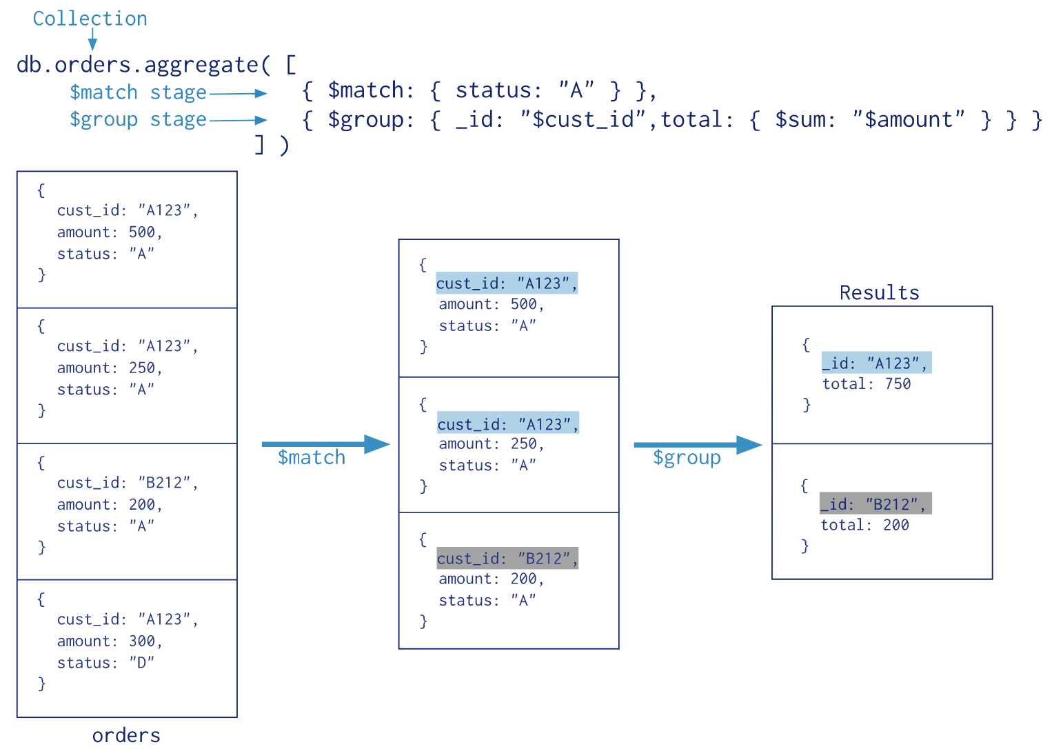
Figure 1: Sample data flows through the Aggregation Pipeline

$match is the first stage In this two stage pipeline. $match will take the entire orders collection as an input and provide as an output a filter with the list of documents where the field, “status” contains the “A” value. The second stage will take these filtered documents as input and perform a grouping of the data to produce the desired query result as an output. While this is a simple example keep in mind that you can build out extremely sophisticated processing pipelines leveraging 100+ operators over 25 different stage classes allowing you to do things like transformations, redacting, sorting, grouping, matching, faceted searches, graph traversals, and joins between different collections to name a few. You can work with data in ways that are just impossible with other distributed databases.

$match는 2개의 stage를 가진 이 pileline의 첫 번째 stage이다. $match는 전체 orders collection을 input으로 사용하고, “status” field가 "A"를 가진 document의 목록을 가진 filter를 output으로 제공한다. 2번째 stage는 이들 filter된 document를 input으로 하고, 원하는 query 결과를 만들기 위해 data를 group화 하여 output으로 한다. 이것은 간단한 예제지만, 변환, 수정, 정렬, 그룹화, 일치, facet 검색, graph 운영, 다른 collection간의 join 등을 할 수 있도록, 25개 이상의 다른 stage에 100개 이상의 연산자를 활용하는 메우 복잡한 process pipeline을 구축할 수 있다는 점을 기억하자. 다른 분산 database에서는 불가능한 방식으로 data를 사용할 수 있다.

With our time-series data we are going to use MongoDB Compass to issue an ad-hoc query that finds the day high price for a given stock. Compass is the GUI tool that allows you to easily explore your data. A useful feature is the ability to visually construct an aggregation pipeline by assembling stages onto a canvas, and then exporting the resultant pipeline as a code for copying and pasting into your app.

우리의 시계열 data를 가지고 MongoDB Compass를 사용하여 특정 주식에 대해 당일 최고가를 찾는 query를 할 것이다. compass는 data를 쉽게 탐색할 수 있는 GUI tool이다. 유용한 기능은 canvas에서 stage를 조합하고, 그 결과로 만들어진 pipeline을 code로 export하여, app에 복사하고 붙여넣음으로써, 집계 pipeline을 시각적으로 구성하는 능력이다.

Finding day high for a given stock

Before diving into the query itself, recall that our StockGen application, described in part 2 of this blog series, produced 1 month of stock price data for 5 stocks we wanted to track. One of the two collections created is called, “StockDocPerMinute” (PerMinute) and it contains a document that represents a minute of data for a specific stock symbol as shown in Figure 2.

query 자체로 들어 가지전에, part 2 에서 설명한 StockGen application이 우리가 추적하려는 5개 주식의 1개월 분량의 주가 data를 생성했다는 점을 기억하자. 생성된 2개의 collection 중 하나인 “StockDocPerMinute” (PerMinute)은 그림 2에서 보듯이 특정 주식 기호에 대한 특정 분(minute)에 대한 data를 나타내는 document를 가지고 있다.

{
            "_id" : ObjectId("5b57a8fae303d36d6df69cd3"),
            "p" : {
                        "0" : 58.75,
                        "1" : 58.75,
                        "2" : 59.45,
...up to…
                        "58" : 58.57,
                        "59" : 59.01
            },
            "symbol" : "FB",
            "d" : ISODate("2018-07-14T00:00:00Z")
}

Figure 2: Sample StockDocPerMinute document

Consider the scenario where the application requests the day high price for a given stock ticker over time. Without the Aggregation Framework this query would have to be either accomplished by retrieving all the data back into the app and using client side code to compute the result, or by defining a map-reduce function in Javascript. Both options are not optimal from a performance or developer productivity perspective.

application이 시간에 따라 주어진 주식 시세에 대해 당일 최고가를 요청하는 시나리오를 생각해 보자. Aggregation Framework가 없다면, 이 query는 모든 data를 app에서 가져와 client측 code를 사용하여 결과를 계산하는 계산하거나, Javascript에서 map-reduce를 정의해야 가능하다. 두 option 모두 성능이나 개발자 생산성 측면에서 최적이 아니다.

Notice the sample document has a subdocument which contains data for an entire minute interval. Using the Aggregation Framework we can easily process this subdocument by transforming the subdocument into an array using the $objectToArray expression, calculating the maximum value and projecting the desired result.

예제 document는 전체 분 간격으로, data를 포함하고 있는 하위 document를 가지고 있다. Aggregation Framework를 사용하면, $objectToArray 를 사용하여, 하위 document를 array로 변경하고, 최대값을 계산하고, 원하는 결과를 예측함으로써, 이 하위 document를 쉽게 처리할 수 있다.

Using MongoDB Compass we can build out the query using the Aggregation Pipeline Builder as follows:

MongoDB Compass를 사용하여, 다음과 같이 Aggregation Pipeline Builder를 사용하는 query를 만들 수 있다.

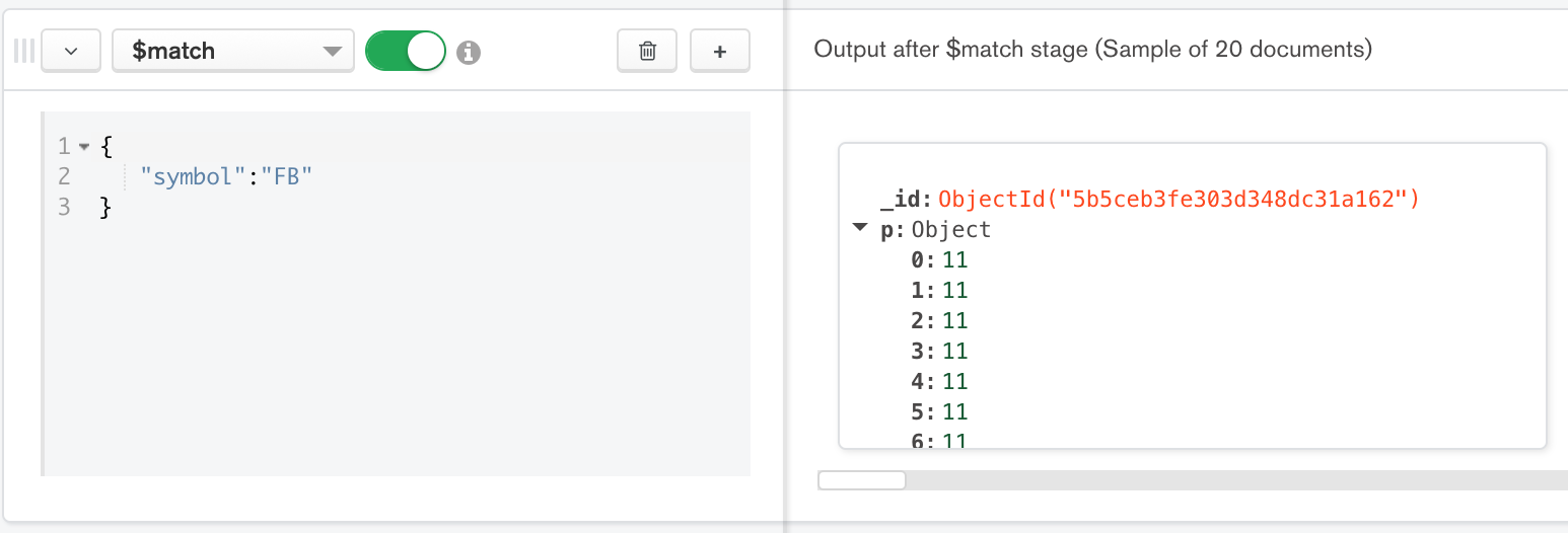
Figure 3: First stage is $match stage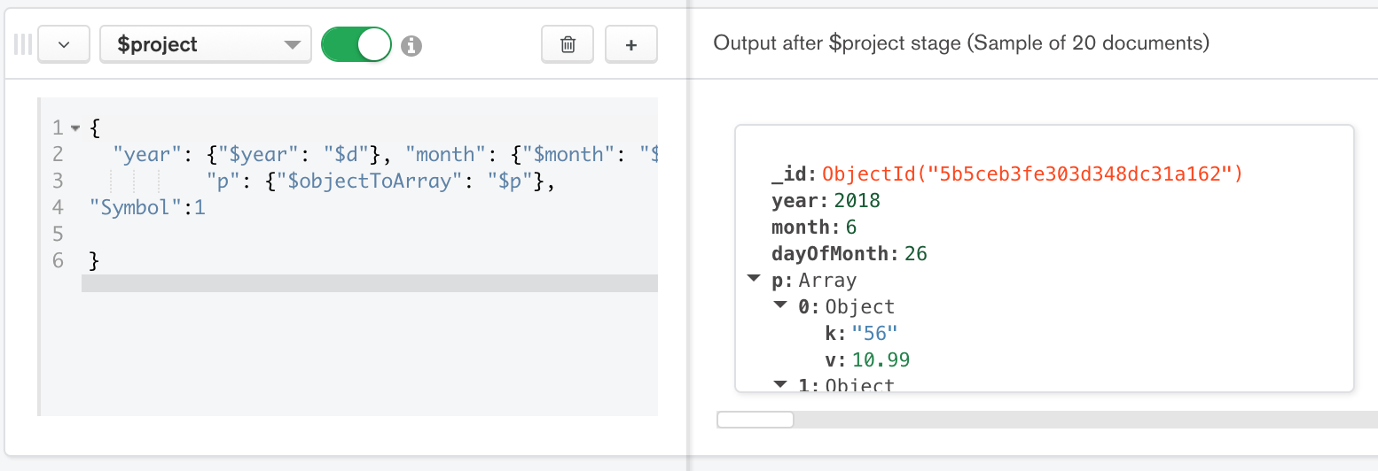

Figure 4: Second stage is the $project stage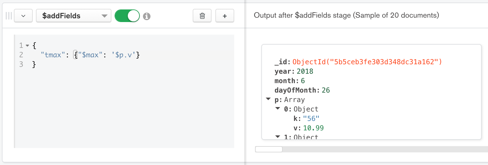

Figure 5: Third stage is the $addFields stage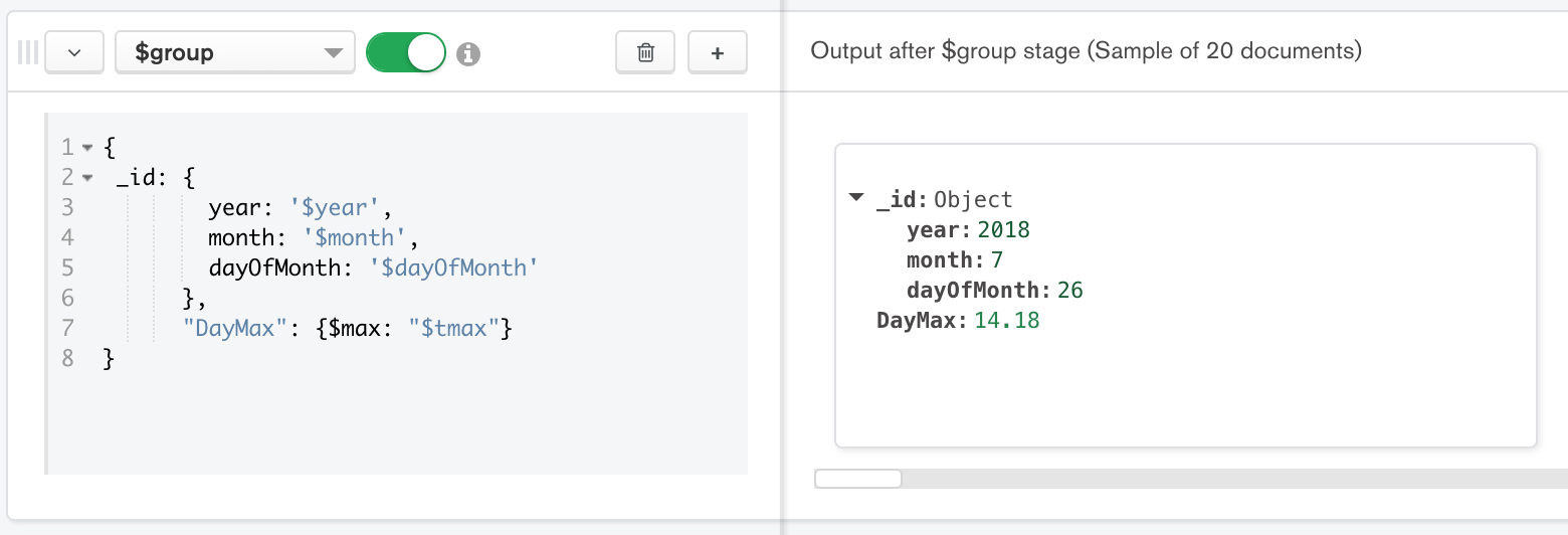

Figure 6: Fourth stage is the $group stage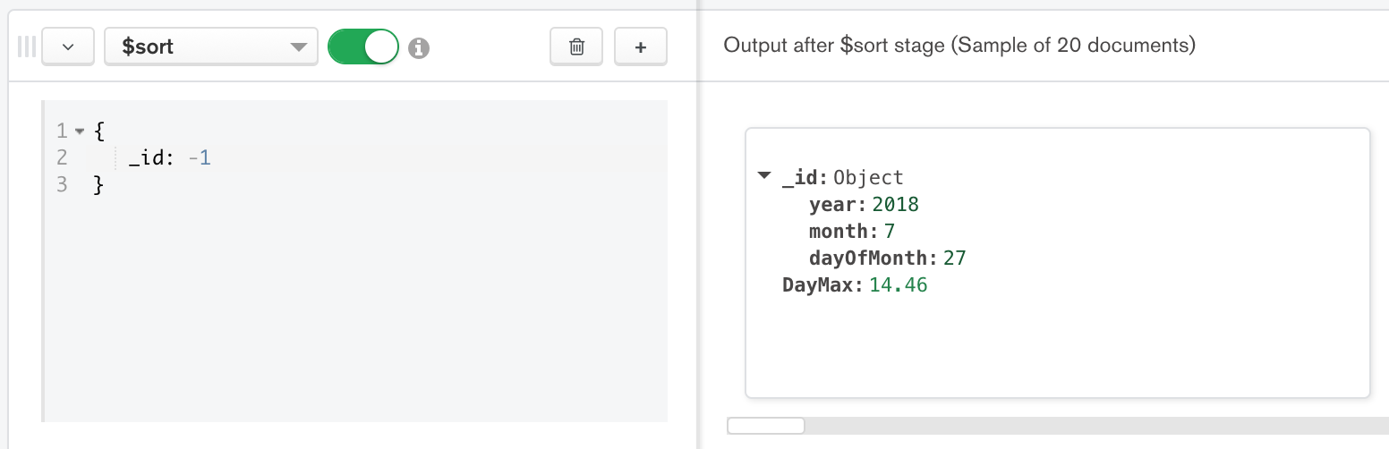

Figure 7: Fifth stage is the $sort stage

We can see the output of the last stage is showing the maximum value per day for each day. Using the aggregation pipeline builder we didn’t need to write a single line of code. For reference, the complete query built by MongoDB Compass in the previous figures is as follows:

마지막 stage의 output이 각 날짜별로 최대값을 보여줌을 알 수 있다. Aggregation Pipeline Builder를 사용하면, code를 한 line씩 작성하지 않아도 된다. 참고로 앞의 그림에서, MongoDB Compass가 작성한 전체 query는 다음과 같다.

db.getCollection('StockDocPerMinute').aggregate([
  { $match: { "symbol" : "FB" } },
  {"$project": 
{ 
"year": {"$year": "$d"}, 
"month": {"$month": "$d"}, 
"dayOfMonth": {"$dayOfMonth": "$d"},
"p": {"$objectToArray": "$p"},
"Symbol":1
} },
    {"$addFields": {"tmax": {"$max": '$p.v'}}},
    {"$group": {
                            _id: {           
                                year: '$year',
                                month: '$month',
                                dayOfMonth: '$dayOfMonth'
                            },
                            "DayMax": {$max: "$tmax"},
                            }
                        },
   {$sort: {_id: -1}}
])

Leveraging Views

MongoDB read-only views can be created from existing collections or from other views. These views act as read-only collections, and are computed on demand during read operations. Since they appear as another collection, you can add a layer of security by restricting access to the underlying collections of the view and just give the client read access to the view. If you want to learn more about access control with Views read the blog post, “Providing Least Privilege Access to MongoDB data”.

기존 collection이나 다른 view에서 MongoDB 읽기 전용 view를 생성할 수 있다. 이 view는 읽기 전용 collection으로 동작하며, read 작업 중에 필요에 따라 계산된다. 이것은 또 다른 collection으로 표시되므로, view의 기반 collection에 대한 access를 제한하거나 view에 client read access를 부여하여, 보안 계층을 추가할 수 있다. view에 대한 access control에 대해 더 많은 정보가 필요하다면, “Providing Least Privilege Access to MongoDB data”를 읽어 보자.

To see how views are created, consider the scenario where the user wants to query stock price history. We can create a view on the StockDocPerMinute collection using the createView syntax as follows:

view를 작성하는 방법을 알아보기 위해 사용자가 주가 기록을 query하는 시나리오를 생각해 보자. 다음과 같이 createView를 사용하여, StockDocPerMinute collection에 view를 생성할 수 있다.

db.createView("ViewStock","StockDocPerMinute", 
[
{"$project": {"p": {"$objectToArray": "$p"}, "d":1, "symbol":1}},
{"$unwind": "$p"},
{"$project": {"_id": 0, "symbol":1,"Timestamp": {
   "$dateFromString": {"dateString":
                           {"$concat": [{"$dateToString":
                                             {"format": "%Y-%m-%dT%H:%M:",
                                              "date": "$d"}},
                                        {"$concat": ["$p.k", "Z"]}]}}}, 
                                        "price":"$p.v"}}
                                    ])

As MongoDB read-only views are materialized at run-time,the latest results are available with each query. Now that the view is defined it can be accessed just like any other collection. For example, to query the first price entry for the “FB” stock using the view we can issue :

run-time에 MongoDB 읽기 전용 view가 구체화되면, 각 query에서 최신 결과를 이용할 수 있다. 이제, view가 정의되었으므로, 다른 collection처럼 access할 수 있다. 예를 들어, view를 사용하여, "FB" 주식의 첫번째 가격을 query하려면 다음과 같이 할 수 있다.

db.ViewStock.find({ "symbol":"FB" } ) .sort({d:-1}).limit(1)

You can also use the aggregation framework with views. Here is the query for all “FB” stock ticker data for a specific day.

view에서 Aggregation Framework를 사용할 수도 있다. 특정 일자의 모든 "FB" 주식 시세 data에 대한 query이다.

db.ViewStock.aggregate({ $match: { 
"symbol":"FB",
 "Timestamp" : { $gte: ISODate("2018-06-26"), $lt: ISODate("2018-06-27") }}},
 { $sort: { "Timestamp": -1 }
})

Querying time-series data with third-party BI Reporting tools

Users may want to leverage existing investments in third-party Business Intelligence Reporting and Analytics tools. To enable these SQL-speaking tools to query data in MongoDB, you can use intermediary service called the MongoDB BI Connector.

사용자가 타사 Business Intelligence Reporting and Analytics tool에서 기존의 투자정보를 활용하려 할 수도 있다. 이들 SQL 사용 tool이 MongoDB data를 query할 수 있게 하려면, MongoDB BI Connector라는 중간 service를 사용할 수 있다.

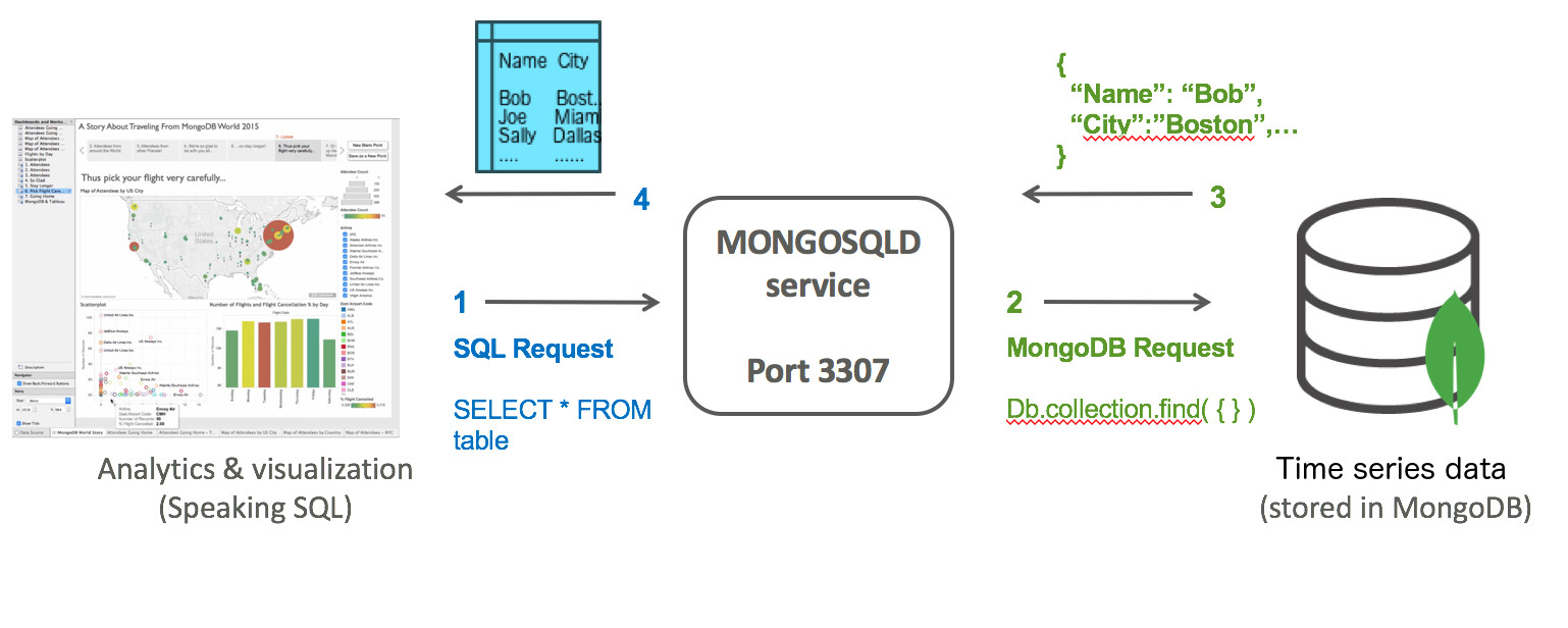
Figure 8: Query MongoDB data with your favorite SQL-based reporting tools using the BI Connector

The BI Connector service presents a port that resembles a MySQL Server to the client application and accepts client connections issuing SQL queries. The BI Connector service then translates these queries into the MongoDB Query Language (MQL) and submits the query to the MongoDB database. Results are returned from MongoDB and flattened into a tabular structure and sent back to the SQL speaking client. This flow is seen in detail in Figure 8.

BI Connector service는 MySQL Server와 유사한 port를 client에 제공하고, SQL query를 실행하는 client 연결을 허용한다.그런 다음, BI Connector services는 이들 query를 MongoDB Query Language(MQL)로 변경하고, MongoDB database에 query를 전송한다. 결과가 MongoDB에서 return되고, table 구조로 전개되어, SQL을 사용하는 client로 다시 전송된다. 자세한 구조는 그림 8에서 볼 수 있다.

To illustrate the MongoDB BI Connector in action, let’s consume our time-series data with Tableau Desktop and the MongoDB BI Connector. Tableau Desktop has a connection option for MongoDB. Using that option and connecting to the port specified in the BI Connector we see that Tableau enumerates the list of tables from our MongoDB database in Figure 9.

MongoDB BI Connector의 실제 동작을 설명하기 위해, ableau Desktop와 MongoDB BI Connector를 사용하여 시계열 data를 살펴보자. Tableau Desktopdms MonogoDB를 위한 연결 option을 가지고 있다. 해당 option을 사용하여, BI Connector에 지정한 port로 연결하면, 그림 9처럼 MongoDB database로 부터 table 목록을 열거하는 것을 볼 수 있다.

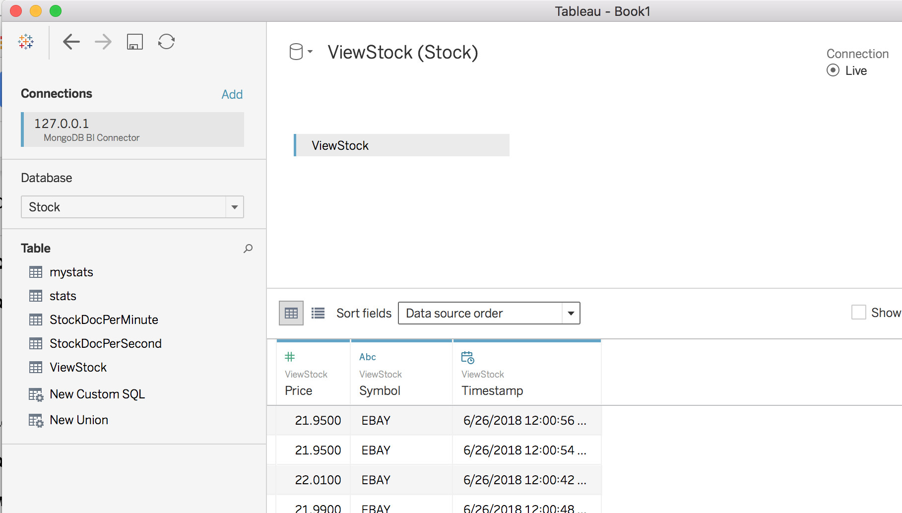
Figure 9: Data Source view in Tableau showing information returned from MongoDB BI Connector

These tables are really our collections in MongoDB. Continuing with the Worksheet view in Tableau we can continue and build out a report showing price over time using the View we created earlier in this document.

이들 table은 실제로 MongoDB의 collection이다. Tableau에서 Worksheet view를 계속해 보면, 앞에서 생성한 view를 사용하여, 시간별 가격을 보여주는 report를 작성할 수 있다.

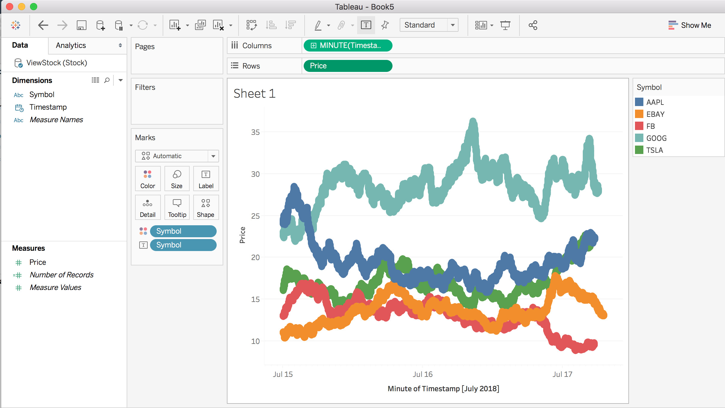
FIgure 10: Sample Tableau worksheet showing price over time

MongoDB Charts

The fastest way to visualize data in MongoDB is with MongoDB Charts. Currently available in Beta it provides users with a web console where they can build and run reports directly from data stored in MongoDB. With Charts there is no special service that needs to run in order to query MongoDB. There is also no need to move the data out or transform it into a different format to be queried. Data can be queried directly as rich documents stored MongoDB. As with other read-only connections, you can connect Charts to secondary replica nodes, therefore isolating analytics and reporting queries from the rest of the cluster serving the operational time series apps. To see how MongoDB Charts can represent data from the StockGen tool, check out the price over time line graph as shown in Figure 11.

MongoDB에서 data를 시각화할 수 있는 가장 빠른 방법은 MongoDB Charts를 사용하는 것이다. 현재 베타 버전을 이용할 수 있으며, MongoDB에 저장된 data에서 직접 report를 작성하고 실행할 수 있는 web console을 사용자에게 제공한다. chart에는 MongoDB를 query하기 위해 실행해야 하는 특별한 service가 없다. 또한 data를 다른 곳으로 이동하거나 query할 다른 형태로 변환할 필요가 없다. data는 MongoDB에 저장된 rich documennt로 바로 query될 수 있다. 다른 읽기 전용 connection과 마찬가지로, chart를 secondary replica node에 연결할 수 있어, 시계열 시리즈의 app을 제공하는 cluster에서 분석 및 report query를 분리할 수 있다. MongoDB Chart가 StockGen tool의 data를 표시하는 방법을 보려면, 그림 11에서 보여주는 시간별 가격 line graph를 확인하자.

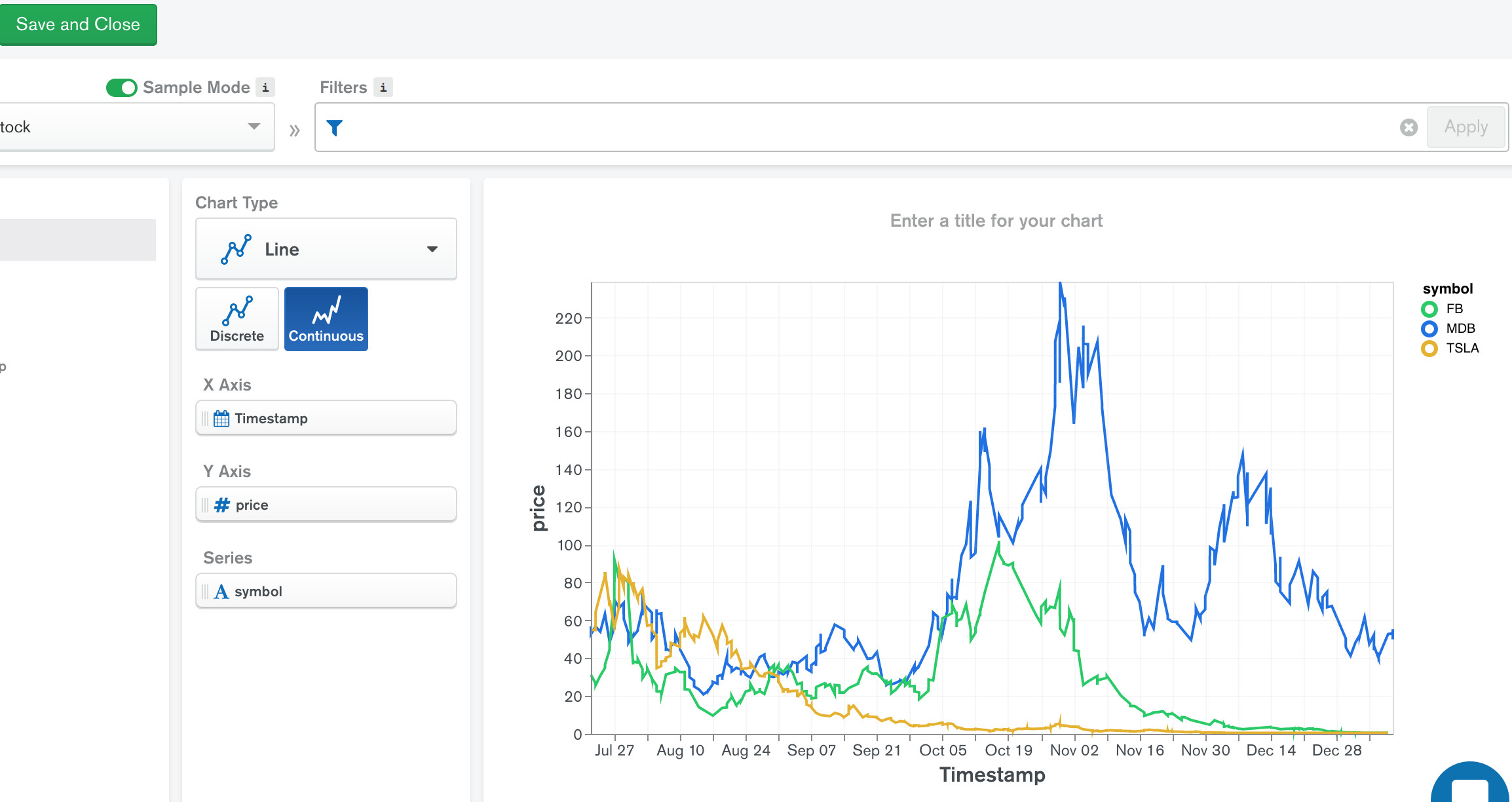
Figure 11: MongoDB Charts showing price over time

At the time of this writing MongoDB Charts is in Beta, therefore details and screenshots may vary from with the final release.

이 글을 스는 시점에서 MongoDB Chart는 베타 버전이므로, 자세한 내용과 screenshot은 최종 버전과 다를 수 있다.

Analytics with MongoDB

In addition to issuing advanced analytics queries with the MongoDB Aggregation Framework, the MongoDB Connector for Apache Spark exposes all of Spark’s libraries, including Scala, Java, Python and R. This enables you to use the Spark analytics engine for big data processing of your time series data extending analytics capabilities of MongoDB even further to perform real-time analytics and machine learning. The connector materializes MongoDB data as DataFrames and Datasets for analysis with machine learning, graph, streaming, and SQL APIs. The Spark connector takes advantage of MongoDB’s aggregation pipeline and rich secondary indexes to extract, filter, and process only the range of data you need! No wasted time extracting and loading data into another database in order to query your MongoDB data using Spark!

MongoDB Aggregation Framework을 사용하여 고급 분석 query를 실행하는 것 외에도, MongoDB Connector for Apache Spark는 Scala, Java, Python, R을 포함한 모든 Spark library를 제공한다. 이를 통해, 시계열 data의 Bigdata 처리에 Spark 분석 엔진을 사용할 수 있고, MongoDB의 분석 기능을 더욱 확장하여 실시간 분석과 Machine Learning을 할 수 있다. connector는 MongoDB data를 Machine Learning, graph, streaming, SQL API로 분석하기 위한 DataFrame과 Dataset으로 구체화한다. Spark connector는 MongoDB의 aggregation pipeliner과 secondary index를 활용하여, 필요한 범위의 data만 추출, filter, 처리한다. Spark를 사용하여 MongoDB를 query하기 위해, 다른 database로 data를 추출하고 load하는데 낭비되는 시간이 없다.

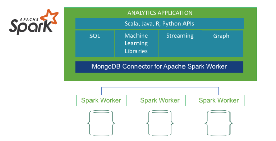
Figure 12: Spark connector for MongoDB

The MongoDB R driver provides developers and statisticians a first class experience with idiomatic, native language access to MongoDB, enterprise authentication, and full support for BSON data types. Using the extensive libraries available to R you could query MongoDB time-series data and determine locally weighted regression as seen in Figure 13.

MongoDB R driver는 개발자와 통계 전문가에게 MongoDB에 대한 관용적, native language 접근, Enterprise 인증, BSON data 유형에 대한 완벽한 지원을 제공한다. R에서 사용할 수 있는 광범위한 library를 사용하면, 그림 13에서 볼 수 있듯이, MongoDB 시계열 data를 query할 수 있고, locally weighted regression을 결정할 수 있다.

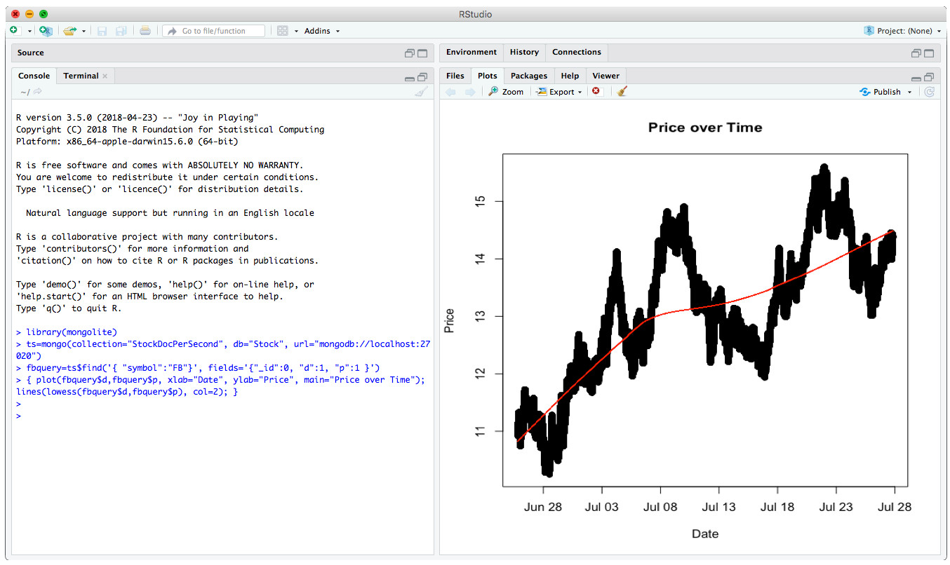
Figure 13: Scatter Plot showing price over time and smoothing of per second data

The R driver for MongoDB is available via the CRAN R Archive. Once installed you can connect to your MongoDB database and return dataframes that can be used in R calculations. The above graph was produced with the following code using R Studio:

R driver for MongoDB 는 CRAN R Archive를 통해 활용할 수 있다. 일단 설치되면, MongoDB에 연결할 수 있고, R에서 사용될 수 있는 dataframe이 return된다. 위의 graph는 R studio를 사용하여 다음과 같은 code로 작성하였다.

library(mongolite)

ts=mongo(collection="StockDocPerSecond", db="Stock", url="mongodb://localhost:27020")

fbquery=ts$find('{ "symbol":"FB"}', fields='{"_id":0, "d":1, "p":1 }')

plot(fbquery$d,fbquery$p, xlab="Date", ylab="Price", main="Price over Time"); 

lines(lowess(fbquery$d,fbquery$p), col=2); 

Summary

While not all data is time-series in nature, a growing percentage of it can be classified as time-series – fueled by technologies that allow us to exploit streams of data in real time rather than in batches. In every industry and in every company there exists the need to query, analyze and report on time-series data. Real business value is derived from the analytics and insights gained from the data. MongoDB enables you to collect, analyze and act on every piece of time-series data in your environment. In this three part series we covered some thought provoking questions with respect to your specific application requirements. In the second blog post we looked at a few different time-series schema designs and their impact on MongoDB performance. Finally we concluded the series showing how to query time series data using the MongoDB Aggregation Framework and MongoDB Compass as well as other methods like using the BI Connector and analytical languages like R.

모든 data가 본질적으로 시계열 data는 아니지만, 점점 더 많은 data가 시계열로 분류될 수 있다. batch가 아닌 실시간으로 data stream을 이용할 수 있는 기술에 의해 가속화된다. 모든 산업과 회사에서 시계열 data를 query, 분석, report할 필요가 있다. 실제 비지니스 가치는 data에서 얻은 분석 및 통찰력에 있다. MongoDB를 사용하면 여러분의 환경에 있는 모든 시게열 data를 수집, 분석, 실행할 수 있다. 이 3개의 게시물에서, 특정 application의 요구사항과 관련하여 몇 가지 생각해봐야 할 질문을 다루었다. 2번째 게시물에서는 몇 가지 시계열 schema design과 그것이 MongoDB 성능에 미치는 영향을 살펴보았다. 마지막으로, MongoDB Aggregation Framework과 MongoDB Compas를 사용하여 시계열 data를 query하는 방법과 BI Connector와 R같은 분석 언어를 사용하는 방법을 보여주면서 마무리지었다.

Prototypes are one thing, but handling terabytes of data efficiently is on a different playing field. With MongoDB it is easy to horizontally scale out time-series workloads. Through the use of replica sets, read-only clients can connect to replica-set secondaries to perform their queries leaving the primary to focus on writes. Write heavy workloads can scale horizontally via sharding. While an in depth analysis of MongoDB architecture is out of scope for these blog posts you can find lots of useful information in the MongoDB Architecture whitepaper.

prototype도 중요하지만, 수 TB의 data를 처리하는 것은 다르다. MongoDB를 사용하면 시계열의 작업량을 쉽게 수평확장할 수 있다. replica set을 사용함으로서, primary는 write에 집중할 수 있도록 하고, 읽기 전용 client는 replica-set secondary에 연결하여 query를 수행할 수 있다. write가 많으며느 sharding을 통해 수평확장할 수 있다. MongoDB architecture에 대한 심층적인 분석은 이 게시물의 범위를 벗어나지만, MongoDB Architecture whitepaper에서 유용한 정보를 많이 볼 수 있다.

The Internet of Things (IoT) use case generates a plethora of time-series data. Larger IoT solutions involve supporting a variety of hardware and software devices for data ingestion, supporting real-time and historical analysis, security, high availability and managing time series data at scale to name a few. MongoDB is powering mission critical IoT applications worldwide. For more information on IoT at MongoDB check out the Internet of Things website.

IoT 사용 사례는 수많은 시계열 data를 생성한다. 대형 IoT 솔루션은 data 수집을 위한 다양한 HW, SW device 지원, 실시간/과거 분석 지원, 보안, 고가용성, 규모에 맞는 시계열 data의 관리 등을 포함한다. MongoDB는 전세계적으로 IoT application을 주도하고 있다, MongoDB의 IoT에 대한 더 많은 정보는 Internet of Things website을 확인해 보자.

원문 : Time Series Data and MongoDB: Part 3 – Querying, Analyzing, and Presenting Time-Series Data